

The DOI matches its Crossref record; 4 of the 4 references it cites were found in a registry or an index.
Modelling species presence‐only data with random forests
Published version of a preprint
Abstract
The random forest (RF) algorithm is an ensemble of classification or regression trees and is widely used, including for species distribution modelling (SDM). Many researchers use implementations of RF in the R programming language with default parameters to analyse species presence‐only data together with ‘background' samples. However, there is good evidence that RF with default parameters does not perform well for such ‘presence‐background' modelling. This is often attributed to the disparity between the number of presence and background samples, also known as 'class imbalance', and several solutions have been proposed. Here, we first set the context: the background sample should be large enough to represent all environments in the region. We then aim to understand the drivers of poor performance of RF when models are fitted to presence‐only species data alongside background samples. We show that 'class overlap' (where both classes occur in the same environment) is an important driver of poor performance, alongside class imbalance. Class overlap can even degrade performance for presence–absence data. We explain, test and evaluate suggested solutions. Using simulated and real presence‐background data, we compare performance of default RF with other weighting and sampling approaches. Our results demonstrate clear evidence of improvement in the performance of RFs when techniques that explicitly manage imbalance are used. We show that these either limit or enforce tree depth. Without compromising the environmental representativeness of the sampled background, we identify approaches to fitting RF that ameliorate the effects of imbalance and overlap and allow excellent predictive performance. Understanding the problems of RF in presence‐background modelling allows new insights into how best to fit models, and should guide future efforts to best deal with such data.
Overview
The claims and statistics of this paper haven’t been checked yet.
Run the check — free, no account needed. It reads the open-access text and checks the sources it cites.
Integrity signals
Registry
Cites
Statistics
Figures
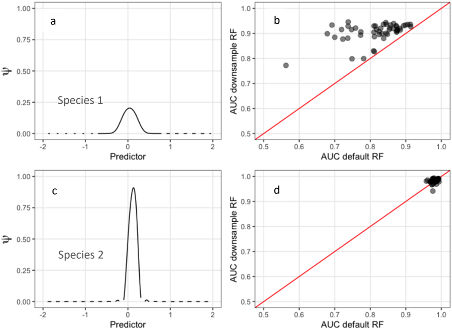
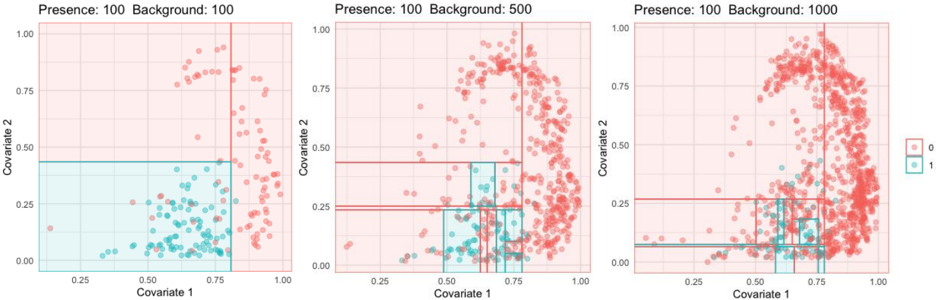
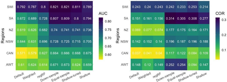
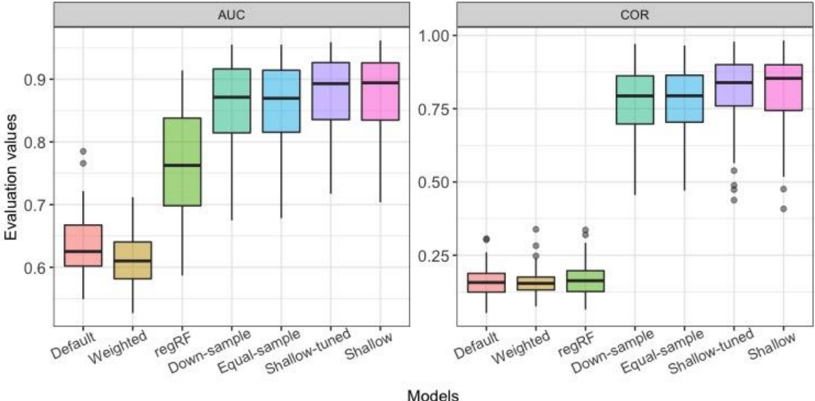
Verification
Claims the paper makes
The claims and statistics of this paper haven’t been checked yet.
Run the check — free, no account needed. It reads the open-access text and checks the sources it cites.
Claims other papers make about this one
Each is checked against this paper’s own text: does it say what the citing paper says it does?
In the citing paper
“Random Forest is the one of the two most popular methods in SDM (Sillero et al., 2021;Valavi et al., 2021;Yaworsky et al., 2020).”
From Predictive modeling for targeted archaeological survey of arsacid period sites in the iranian borderland region of the araxes river valley (2026) · cites this paper as Valavi et al., 2021
In the citing paper
“It is, however, prone to overfitting because the decision trees could infinitely deepen to the level of individual observations (Valavi et al., 2021;Yaworsky et al., 2020).”
From Predictive modeling for targeted archaeological survey of arsacid period sites in the iranian borderland region of the araxes river valley (2026) · cites this paper as Valavi et al., 2021
Self-check
Percentages, sums and reported differences re-computed from the paper’s own numbers.
The self-check needs the paper’s full text.
Citations
Cites
Kuhn, M., & Johnson, K. (2013) · doi:10.1007/978-1-4614-6849-3 · Cited by 6,788
Random forests for classification in ecology
Cutler, D. R., Edwards, T. C., Beard, K. H., Cutler, A., Hess, K. T., Gibson, J., & Lawler, J. J. (2007) · Ecology · doi:10.1890/07-0539.1 · Cited by 4,950
Strobl, C., Malley, J., & Tutz, G. (2009) · Psychological Methods · doi:10.1037/a0016973 · Cited by 2,583
Learning from imbalanced data: open challenges and future directions
Krawczyk, B. (2016) · Progress in Artificial Intelligence · doi:10.1007/s13748-016-0094-0 · Cited by 2,459
Research works printed but not linked: 56
- Ali A., 2015, Classification with class imbalance problem: a review, Int. J. Adv. Soft Comput. Appl., 7, 176
- 10.1126/sciadv.aat4858 · DOI
- 10.1111/j.2041-210X.2011.00172.x · DOI · Paper page
- 10.1007/978-3-642-52307-6_8 · DOI
- 10.1023/A:1010933404324 · DOI · Paper page
- Chen C., 2004, Using random forest to learn imbalanced data, 1
- Cieslak D. A., 2008, Learning decision trees for unbalanced data, Daelemans, W. et al. (eds), Joint European conference on machine learning and knowledge discovery in databases, 241
- 10.1007/s10618-011-0222-1 · DOI
- Demšar J., 2006, Statistical comparisons of classifiers over multiple data sets, J. Mach. Learn. Res., 7
- Denil M., 2010, Overlap versus imbalance, Advances in artificial intelligence lecture notes in computer science, 220
- Drummond C., 2000, Exploiting the cost (In) sensitivity of decision tree splitting criteria, ICML, 8
- 10.1201/9780429246593 · DOI · Paper page
- Elith J., 2019, Machine learning, random forests and boosted regression trees, Brennan, L. et al. (eds), Quantitative analyses in wildlife science wildlife management and conservation, 281
- 10.1111/j.2006.0906-7590.04596.x · DOI · Paper page
- 10.17161/bi.v15i2.13384 · DOI
- 10.1007/s10980-009-9341-0 · DOI
- 10.1111/2041-210X.12242 · DOI
- 10.1017/CBO9780511810602 · DOI
- 10.1016/j.ecolmodel.2012.03.007 · DOI
- 10.1139/cjfr-2014-0562 · DOI
- García S., 2008, An extension on ‘statistical comparisons of classifiers over multiple data sets' for all pairwise comparisons, J. Mach. Learn. Res., 9, 2677
- 10.1111/geb.12268 · DOI
- 10.1016/S0304-3800(02)00204-1 · DOI · Paper page
- 10.1017/9781139028271 · DOI
- Hastie T., 2009, The elements of statistical learning: data mining, inference and prediction, 10.1007/978-0-387-84858-7 · DOI · Paper page
- 10.1109/TKDE.2008.239 · DOI · Paper page
- Japkowicz N., 2003, Class imbalances: are we focusing on the right issue, Workshop on learning from imbalanced data sets II
- 10.3233/IDA-2002-6504 · DOI · Paper page
- 10.1109/CIDU.2012.6382186 · DOI
- 10.1186/1472-6947-11-51 · DOI
- Kujala H., 2015, Identifying conservation priorities and assessing impacts and trade‐offs of potential future development in the Lower Hunter Valley in New South Wales. Univ. of Melbourne, Melbourne, Victoria, 106
- 10.1111/ecog.01388 · DOI
- Liaw A., 2002, Classification and regression by randomForest, R News, 2, 18
- 10.1016/j.ecolmodel.2012.07.003 · DOI
- 10.1145/3347711 · DOI
- 10.3414/ME00-01-0052 · DOI
- 10.1111/ecog.00845 · DOI
- 10.1111/j.1600-0587.2011.07157.x · DOI
- Mthembu L., 2008, A note on the separability index, arXiv:0812.1107. · arXiv
- 10.1086/587826 · DOI · Paper page
- 10.1016/S0304-3800(00)00322-7 · DOI
- 10.1890/07-2153.1 · DOI · Paper page
- Prati R. C., 2004, Class imbalances versus class overlapping: an analysis of a learning system behavior, Mexican international conference on artificial intelligence, 312
- Probst P., 2019, Tunability: importance of hyperparameters of machine learning algorithms, J. Mach. Learn. Res., 20, 1
- Probst P., 2019, Hyperparameters and tuning strategies for random forest, Wiley Interdisciplinary Reviews: Data Mining and Knowledge Discovery, 9, e1301
- Rabinowitz D., 1981, Seven forms of rarity, The biological aspects of rare plant conservation (ed. by H. Synge). Wiley, 205
- 10.1111/2041-210X.12352 · DOI
- 10.1111/ecog.02881 · DOI · Paper page
- 10.1111/ddi.12698 · DOI
- 10.1002/ece3.2332 · DOI
- 10.1029/2019WR024884 · DOI
- 10.1186/1471-2105-8-25 · DOI
- 10.1002/ecm.1486 · DOI · Paper page
- 10.1214/10-AOAS331 · DOI
- Wright M. N., 2017, ranger: a fast implementation of random forests for high dimensional data in C++ and R, J. Stat. Softw., 77, 1, 10.18637/jss.v077.i01 · DOI
- 10.1016/j.ecoinf.2019.05.003 · DOI
Cited by
Sorted by citations
Wang, J., Soroush, M., Maziar, S., & Khazraee, E. (2026) · Journal of Archaeological Method and Theory · doi:10.1007/s10816-025-09733-5 · Cited by 3
Metadata
- Authors
- Valavi, R., Elith, J., Lahoz‐Monfort, J. J., & Guillera‐Arroita, G.
- Venue
- Ecography
- Publisher
- Wiley
- Published
- 2021-10-27
- Volume
- 44
- Issue
- 12
- Pages
- 1731-1742
- ISSN
- 0906-7590
- 1600-0587
- Cited by
- 307
- References
- 4
- Language
- en
About these checks
Registry, retraction, Cites and statistics results are computed, not judged, with one exception: a printed reference that no index lists is read once by a model before it counts as a citation error. Claims are extracted by a model and kept only when their quote appears verbatim in the text; each cited source is then checked, with a model’s help, for whether it says what the claim relies on. Those verdicts can be wrong — read the claim’s quote and the cited source before relying on one.
Statistics and arithmetic are recomputed, not judged.
Confidence bands are shown only for fields calibrated on our annotated test set. None is calibrated yet, so no band is shown.
What counts as a claim ›How we measure confidence ›How we check this ›
Are you an author, or do you see a problem with this page? Request a review
