CoChat

The DOI matches its Crossref record; 70 of the 70 references it cites were found in a registry or an index.

Deep neural network processing of DEER data

Open access

Abstract

Deep neural networks successfully solve Fredholm equations and extract molecular-scale distance distributions from EPR data.

Overview

The claims and statistics of this paper haven’t been checked yet.

Free: it reads the open-access text and checks the first 5 claims that cite a source we can check. Create a free account to check every claim.

A few free checks a day · papers already verified open instantly · results are public

Integrity signals

Registry

Crossref · 10.1126/sciadv.aat5218

Cites

70 of 70 references verified0 citation errors · 0 not checkable

Statistics

Figures

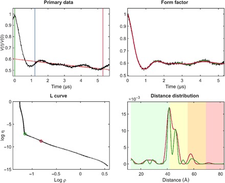
Fig. 1 Standard Tikhonov regularization processing, illustrated using site pair V96C/I143C in the lumenal loop of a double mutant of LHCII, with iodoacetamido-PROXYL spin labels attached to the indicated cysteines (64). For the primary data (top left), the zero time (green vertical line) is determined using moment analysis in the vicinity of the intensity maximum. The optimal starting time for background fitting (blue vertical line) is determined by minimizing probability density at the maximum distance. Data have been cut by 400 ns at the end (red vertical line) to minimize the influence of the artifact arising from overlapping pump and observe pulse excitation bands. The stretched exponential background fit is shown as a solid red line (where fitted) and as a dotted red line (where extrapolated). The background-corrected data (form factor, black) are shown in the top right panel together with fits using the regularization parameter corresponding to the origin distance criterion (red) and maximum curvature criterion (green). These two choices are also indicated in the L-curve (bottom left). The bottom right panel shows distance distributions computed with these two regularization parameters in matching color. Pastel background shading indicates distance ranges where the shape of the distribution is expected to be reliable (green), where mean distances and widths are expected to be reliable (yellow), where only mean distances are expected to be reliable (orange), and where data should not be interpreted (red). These ranges are derived from the duration of the primary data (7).
Fig. 1 Standard Tikhonov regularization processing, illustrated using site pair V96C/I143C in the lumenal loop of a double mutant of LHCII, with iodoacetamido-PROXYL spin labels attached to the indicated cysteines (64). For the primary data (top left), the zero time (green vertical line) is determined using moment analysis in the vicinity of the intensity maximum. The optimal starting time for background fitting (blue vertical line) is determined by minimizing probability density at the maximum distance. Data have been cut by 400 ns at the end (red vertical line) to minimize the influence of the artifact arising from overlapping pump and observe pulse excitation bands. The stretched exponential background fit is shown as a solid red line (where fitted) and as a dotted red line (where extrapolated). The background-corrected data (form factor, black) are shown in the top right panel together with fits using the regularization parameter corresponding to the origin distance criterion (red) and maximum curvature criterion (green). These two choices are also indicated in the L-curve (bottom left). The bottom right panel shows distance distributions computed with these two regularization parameters in matching color. Pastel background shading indicates distance ranges where the shape of the distribution is expected to be reliable (green), where mean distances and widths are expected to be reliable (yellow), where only mean distances are expected to be reliable (orange), and where data should not be interpreted (red). These ranges are derived from the duration of the primary data (7).CC BY · PubMed Central
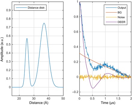
Fig. 2 One of the millions of synthetic DEER data sets, generated using Spinach (25) and used for neural network training in this work. (Left) Randomly generated distance distribution. (Right) The corresponding DEER form factor (purple), a randomly generated noise track (yellow), a randomly generated intermolecular background signal (red, marked BG), and the resulting “experimental” DEER signal (blue). a.u., arbitrary units.
Fig. 2 One of the millions of synthetic DEER data sets, generated using Spinach (25) and used for neural network training in this work. (Left) Randomly generated distance distribution. (Right) The corresponding DEER form factor (purple), a randomly generated noise track (yellow), a randomly generated intermolecular background signal (red, marked BG), and the resulting “experimental” DEER signal (blue). a.u., arbitrary units.CC BY · PubMed Central
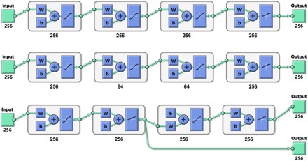
Fig. 3 Schematic diagrams (produced by MATLAB) of the three types of neural network topologies explored in this work, using four-layer networks as an example. W block indicates multiplication by the weight matrix and b block indicates the addition of a bias vector. (Top) Fully connected full-width network. (Middle) Fully connected network with choke points. (Bottom) Functionally separated network with some layers explicitly dedicated to background rejection and others to interpretation—during the training process, the first output is the DEER form factor, and the second output is the distance probability density function.
Fig. 3 Schematic diagrams (produced by MATLAB) of the three types of neural network topologies explored in this work, using four-layer networks as an example. W block indicates multiplication by the weight matrix and b block indicates the addition of a bias vector. (Top) Fully connected full-width network. (Middle) Fully connected network with choke points. (Bottom) Functionally separated network with some layers explicitly dedicated to background rejection and others to interpretation—during the training process, the first output is the DEER form factor, and the second output is the distance probability density function.CC BY · PubMed Central
Fig. 4 Distance distribution recovery performance illustration for a five-layer feedforward neural network, fully connected, with 256 neurons per layer. All inner layers have hyperbolic tangent transfer functions; the last layer has the strictly positive logistic sigmoid transfer function.
Fig. 4 Distance distribution recovery performance illustration for a five-layer feedforward neural network, fully connected, with 256 neurons per layer. All inner layers have hyperbolic tangent transfer functions; the last layer has the strictly positive logistic sigmoid transfer function.CC BY · PubMed Central
Fig. 5 DEER form factor recovery performance illustration for a six-layer feedforward neural network, fully connected, with 256 neurons per layer. All layers have hyperbolic tangent transfer functions.
Fig. 5 DEER form factor recovery performance illustration for a six-layer feedforward neural network, fully connected, with 256 neurons per layer. All layers have hyperbolic tangent transfer functions.CC BY · PubMed Central
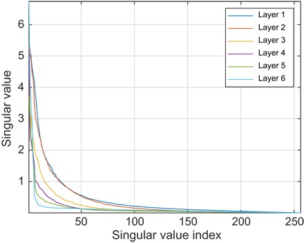
Fig. 6 Singular values of the weight matrices in a six-layer feedforward neural network, fully connected, with 256 neurons per layer, and trained as described in the main text. All inner layers have hyperbolic tangent transfer functions; the last layer has the strictly positive logistic sigmoid transfer function.
Fig. 6 Singular values of the weight matrices in a six-layer feedforward neural network, fully connected, with 256 neurons per layer, and trained as described in the main text. All inner layers have hyperbolic tangent transfer functions; the last layer has the strictly positive logistic sigmoid transfer function.CC BY · PubMed Central
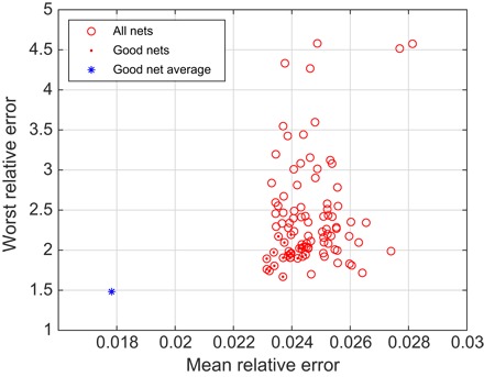
Fig. 7 Performance of an ensemble of 100 five-layer neural networks on a previously unseen database. Each of the networks was started from a different random initial guess and trained in a different randomly generated database. Red dots indicate the good networks that are better than the median on both the mean relative error and the worst relative error. The blue asterisk is the performance of the average output of the good networks.
Fig. 7 Performance of an ensemble of 100 five-layer neural networks on a previously unseen database. Each of the networks was started from a different random initial guess and trained in a different randomly generated database. Red dots indicate the good networks that are better than the median on both the mean relative error and the worst relative error. The blue asterisk is the performance of the average output of the good networks.CC BY · PubMed Central
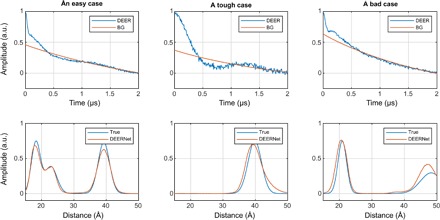
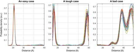
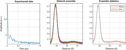
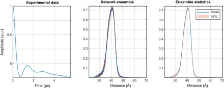
Fig. 8 Network ensemble performance illustration. Easy (left), tough (middle), and worst-case (right) agreement on the training set data. The variation in the outputs of different neural networks within the ensemble is a measure of the uncertainty in their output (63) when the training databases are comprehensive.
Fig. 8 Network ensemble performance illustration. Easy (left), tough (middle), and worst-case (right) agreement on the training set data. The variation in the outputs of different neural networks within the ensemble is a measure of the uncertainty in their output (63) when the training databases are comprehensive.CC BY · PubMed Central
Fig. 9 A demonstration that deep neural networks learn to be Fredholm solvers rather than model fitters. Presenting a data set with four distances to networks trained on the database with at most three distances yields the right answer with high confidence. All networks in the ensemble return four peaks.
Fig. 9 A demonstration that deep neural networks learn to be Fredholm solvers rather than model fitters. Presenting a data set with four distances to networks trained on the database with at most three distances yields the right answer with high confidence. All networks in the ensemble return four peaks.CC BY · PubMed Central
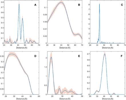
Fig. 10 Distance distributions obtained by Tikhonov regularization (blue lines) and uncertainties estimated by the DeerAnalysis validation tool (pink areas) for the six experimental test cases. (A) Site pair V96C/I143C in the lumenal loop of a double mutant of LHCII, with iodoacetamido-PROXYL spin labels attached to the indicated cysteines (64); (B) site pair S3C/S34C in the N-terminal domain of a double mutant of the LHCII monomers, with iodoacetamido-PROXYL spin labels attached to the indicated cysteines (64); (C) end-labeled oligo(para-phenyleneethynylene)—a rigid linear molecule described as compound 3a in (37); (D) [2]catenane (a pair of large interlocked rings) with a nitroxide spin label on each ring described as sample II in (65); (E) pairs of nitroxide radicals tethered to the surface of gold nanoparticles, with the thiol tether attachment points diffusing on the surface of the nanoparticle, sample Au3 after solvolysis and heating in (66); (F) rigid molecular triangle labeled with nitroxide radicals on two corners out of three, sample B11inv in (16).
Fig. 10 Distance distributions obtained by Tikhonov regularization (blue lines) and uncertainties estimated by the DeerAnalysis validation tool (pink areas) for the six experimental test cases. (A) Site pair V96C/I143C in the lumenal loop of a double mutant of LHCII, with iodoacetamido-PROXYL spin labels attached to the indicated cysteines (64); (B) site pair S3C/S34C in the N-terminal domain of a double mutant of the LHCII monomers, with iodoacetamido-PROXYL spin labels attached to the indicated cysteines (64); (C) end-labeled oligo(para-phenyleneethynylene)—a rigid linear molecule described as compound 3a in (37); (D) [2]catenane (a pair of large interlocked rings) with a nitroxide spin label on each ring described as sample II in (65); (E) pairs of nitroxide radicals tethered to the surface of gold nanoparticles, with the thiol tether attachment points diffusing on the surface of the nanoparticle, sample Au3 after solvolysis and heating in (66); (F) rigid molecular triangle labeled with nitroxide radicals on two corners out of three, sample B11inv in (16).CC BY · PubMed Central
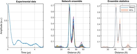
Fig. 11 DEERNet performance on sample I: A site pair V96C/I143C in the lumenal loop of a double mutant of LHCII, with iodocateamido-PROXYL spin labels attached to the indicated cysteines (64). Residue 96 is located in the lumenal loop, and residue 143 is a structurally rigid “anchor” position in the protein core. In agreement with the results reported in the original paper, a bimodal distance distribution is measured—indicating flexibility in the lumenal loop. The low-confidence peak around 57 Å likely results from protein aggregation.
Fig. 11 DEERNet performance on sample I: A site pair V96C/I143C in the lumenal loop of a double mutant of LHCII, with iodocateamido-PROXYL spin labels attached to the indicated cysteines (64). Residue 96 is located in the lumenal loop, and residue 143 is a structurally rigid “anchor” position in the protein core. In agreement with the results reported in the original paper, a bimodal distance distribution is measured—indicating flexibility in the lumenal loop. The low-confidence peak around 57 Å likely results from protein aggregation.CC BY · PubMed Central
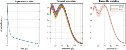
Fig. 12 DEERNet performance on sample II: A site pair S3C/S34C in the N-terminal domain of a double mutant of the LHCII, with iodoacetamido-PROXYL spin labels attached to the indicated cysteines (64). The data stem from LHCIII monomers. Residue 3 is located in the very flexible N-terminal region, while residue 34 is located in the structured part of the N-terminal domain.
Fig. 12 DEERNet performance on sample II: A site pair S3C/S34C in the N-terminal domain of a double mutant of the LHCII, with iodoacetamido-PROXYL spin labels attached to the indicated cysteines (64). The data stem from LHCIII monomers. Residue 3 is located in the very flexible N-terminal region, while residue 34 is located in the structured part of the N-terminal domain.CC BY · PubMed Central
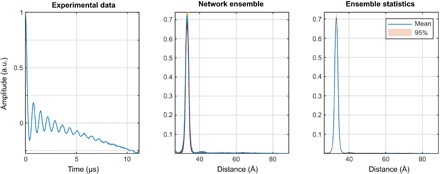
Fig. 13 DEERNet performance on sample III: End-labeled oligo(para-phenyleneethynylene)—a rigid linear molecule described as compound 3a in (37). The maximum and the width of the distance distribution are in close agreement with the Tikhonov regularization results, whereas the expected skew of the distribution is not reproduced. Notably, there are no low-intensity artifacts that the Tikhonov method produces around the baseline.
Fig. 13 DEERNet performance on sample III: End-labeled oligo(para-phenyleneethynylene)—a rigid linear molecule described as compound 3a in (37). The maximum and the width of the distance distribution are in close agreement with the Tikhonov regularization results, whereas the expected skew of the distribution is not reproduced. Notably, there are no low-intensity artifacts that the Tikhonov method produces around the baseline.CC BY · PubMed Central
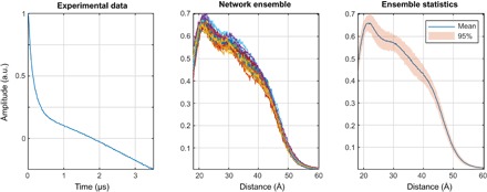
Fig. 14 DEERNet performance on Sample IV: [2]catenane (a pair of large interlocked rings) with a nitroxide spin label on each ring. The distance distribution is in line with rough statistical estimates [Figure 5 in (65)], but there are fewer clumping artifacts compared to the output of the automatic Tikhonov regularization procedure. Within the Tikhonov framework, a manual regularization coefficient adjustment away from the corner of the L-curve is necessary to produce a distribution free of clumping artifacts.
Fig. 14 DEERNet performance on Sample IV: [2]catenane (a pair of large interlocked rings) with a nitroxide spin label on each ring. The distance distribution is in line with rough statistical estimates [Figure 5 in (65)], but there are fewer clumping artifacts compared to the output of the automatic Tikhonov regularization procedure. Within the Tikhonov framework, a manual regularization coefficient adjustment away from the corner of the L-curve is necessary to produce a distribution free of clumping artifacts.CC BY · PubMed Central
Fig. 15 DEERNet performance on sample V: Pairs of nitroxide radicals tethered to the surface of gold nanoparticles, with the thiol tether attachment points diffusing on the surface of the nanoparticle (66). Note the markedly better performance relative to the Tikhonov method: The complete absence of clumping artifacts and the remarkable match to the analytical model—down to the maximum exhibited by the broad feature around 35 Å.
Fig. 15 DEERNet performance on sample V: Pairs of nitroxide radicals tethered to the surface of gold nanoparticles, with the thiol tether attachment points diffusing on the surface of the nanoparticle (66). Note the markedly better performance relative to the Tikhonov method: The complete absence of clumping artifacts and the remarkable match to the analytical model—down to the maximum exhibited by the broad feature around 35 Å.CC BY · PubMed Central
Fig. 16 Tikhonov distance distribution analysis for pairs of nitroxide radicals tethered to the surface of gold nanoparticles, with the thiol tether attachment points diffusing on the surface of the nanoparticle [sample Au3 after solvolysis and heating in (66)]. Green lines correspond to a model fit assuming a Gaussian distribution of distances and a homogeneous distribution of the biradicals on spherical nanoparticles with a Gaussian distribution of radii. Blue lines correspond to Tikhonov regularization with the regularization parameter in the L-curve corner as suggested by DeerAnalysis. Red lines correspond to Tikhonov regularization with a larger regularization parameter corresponding to the second L-curve corner. (A) Fits of the background-corrected DEER data (black). (B) Distance distributions. (C) L-curve and the two points selected for Tikhonov distance distribution analysis.
Fig. 16 Tikhonov distance distribution analysis for pairs of nitroxide radicals tethered to the surface of gold nanoparticles, with the thiol tether attachment points diffusing on the surface of the nanoparticle [sample Au3 after solvolysis and heating in (66)]. Green lines correspond to a model fit assuming a Gaussian distribution of distances and a homogeneous distribution of the biradicals on spherical nanoparticles with a Gaussian distribution of radii. Blue lines correspond to Tikhonov regularization with the regularization parameter in the L-curve corner as suggested by DeerAnalysis. Red lines correspond to Tikhonov regularization with a larger regularization parameter corresponding to the second L-curve corner. (A) Fits of the background-corrected DEER data (black). (B) Distance distributions. (C) L-curve and the two points selected for Tikhonov distance distribution analysis.CC BY · PubMed Central
Fig. 17 DEERNet performance on sample VI: A rigid molecular triangle labeled with nitroxide radicals on two out of three corners (16).
Fig. 17 DEERNet performance on sample VI: A rigid molecular triangle labeled with nitroxide radicals on two out of three corners (16).CC BY · PubMed Central
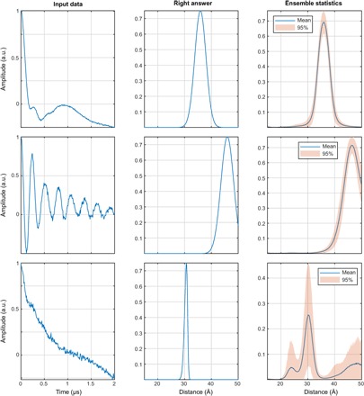
Fig. 18 A demonstration of exchange coupling resilience. The networks were trained on the database where each DEER trace has an exchange coupling randomly selected within the ±5-MHz interval (top row, J = –1.9 MHz; middle row, J = +2.9 MHz; bottom row, J = –3.6 MHz) and all other parameters as described in the “Training database generation” section. More than 99% of the training data set (including distributions with multiple distance peaks) produces the results of the kind shown in the top and middle panels—fast exchange oscillations are rejected and correct distance distributions are produced. With very noisy data (bottom), the networks duly report being highly uncertain.
Fig. 18 A demonstration of exchange coupling resilience. The networks were trained on the database where each DEER trace has an exchange coupling randomly selected within the ±5-MHz interval (top row, J = –1.9 MHz; middle row, J = +2.9 MHz; bottom row, J = –3.6 MHz) and all other parameters as described in the “Training database generation” section. More than 99% of the training data set (including distributions with multiple distance peaks) produces the results of the kind shown in the top and middle panels—fast exchange oscillations are rejected and correct distance distributions are produced. With very noisy data (bottom), the networks duly report being highly uncertain.CC BY · PubMed Central

Verification

Claims the paper makes

The claims and statistics of this paper haven’t been checked yet.

Free: it reads the open-access text and checks the first 5 claims that cite a source we can check. Create a free account to check every claim.

A few free checks a day · papers already verified open instantly · results are public

Self-check

Percentages, sums and reported differences re-computed from the paper’s own numbers.

The self-check needs the paper’s full text.

Citations

Cites

Show all 70 references

Research works printed but not linked: 2

  1. A. D. Milov, K. M. Salikhov, M. D. Shirov, Use of the double resonance in electron spin echo method for the study of paramagnetic center spatial distribution in solids. Fizika Tverdogo Tela 23, 975–982 (1981).
  2. 10.1002/1521-3927(20020301)23:4<227::aid-marc227>3.0.co;2-d · doi:10.1002/1521-3927(20020301)23:4<227::aid-marc227>3.0.co;2-d

Cited by

See all 223

Metadata

Authors
Worswick, S. G., Spencer, J. A., Jeschke, G., & Kuprov, I.
Affiliations
  • University of Southampton (GB)
  • ETH Zurich (CH)
Corresponding author
Kuprov, Ilya
Venue
Science Advances
Published
2018-08-03
Volume
4
Issue
8
Pages
eaat5218-eaat5218
ISSN
2375-2548 (ISSN-L)
OpenAlex
W2888649302
Cited by
212
References
70
Citations by year
2026: 13 · 2025: 26 · 2024: 33 · 2023: 36 · 2022: 47 · 2021: 30 · 2020: 11 · 2019: 15 · 2018: 1
FWCI
7.44
Type
journal article
Language
en
Open access
Licence
cc-by
Locations
  • Science Advances (publishedVersion, cc-by)
  • Europe PMC (PubMed Central) (publishedVersion, cc-by)
  • PubMed Central (publishedVersion, cc-by)
  • PubMed (publishedVersion)
  • ePrints Soton (University of Southampton) (submittedVersion)
  • Repository for Publications and Research Data (ETH Zurich) (submittedVersion, cc-by)
  • ETH Zürich Research Collection (cc-by)
Funders
Engineering and Physical Sciences Research Council (EP/N006895/1)
Topics
  • Physical Sciences › Chemistry › Spectroscopy › Electron Spin Resonance Studies
  • Physical Sciences › Materials Science › Electronic, Optical and Magnetic Materials › Magnetism in coordination complexes
  • Physical Sciences › Chemistry › Spectroscopy › Advanced NMR Techniques and Applications
Keywords
double electron-electron resonance, artificial neural networks, model-independent analysis, distance distribution, exchange interaction, synthetic training data, uncertainty estimation, PELDOR, spinach

About these checks

Registry, retraction, Cites and statistics results are computed, not judged, with one exception: a printed reference that no index lists is read once by a model before it counts as a citation error. Claims are extracted by a model and kept only when their quote appears verbatim in the text; each cited source is then checked, with a model’s help, for whether it says what the claim relies on. Those verdicts can be wrong — read the claim’s quote and the cited source before relying on one.

Statistics and arithmetic are recomputed, not judged.

Confidence bands are shown only for fields calibrated on our annotated test set. None is calibrated yet, so no band is shown.

What counts as a claim ›How we measure confidence ›How we check this ›

Are you an author, or do you see a problem with this page? Request a review

Data sources

Bibliographic data: Semantic Scholar, OpenAlex, Crossref.

Contains information from the Semantic Scholar Academic Graph Datasets, made available under the ODC Attribution License (ODC-BY 1.0).

Semantic Scholar’s data is described in: Kinney, R., et al. (2023). The Semantic Scholar Open Data Platform. arXiv:2301.10140.