

The DOI matches its Crossref record; 6 of the 6 references it cites were found in a registry or an index.
GraphAligner: rapid and versatile sequence-to-graph alignment
Open accessPublished version of a preprint
Abstract
Genome graphs can represent genetic variation and sequence uncertainty. Aligning sequences to genome graphs is key to many applications, including error correction, genome assembly, and genotyping of variants in a pangenome graph. Yet, so far, this step is often prohibitively slow. We present GraphAligner, a tool for aligning long reads to genome graphs. Compared to the state-of-the-art tools, GraphAligner is 13x faster and uses 3x less memory. When employing GraphAligner for error correction, we find it to be more than twice as accurate and over 12x faster than extant tools.Availability: Package manager: https://anaconda.org/bioconda/graphaligner and source code: https://github.com/maickrau/GraphAligner
Overview
The claims and statistics of this paper haven’t been checked yet.
Run the check — free, no account needed. It reads the open-access text and checks the sources it cites.
Integrity signals
Registry
Cites
Statistics
Figures
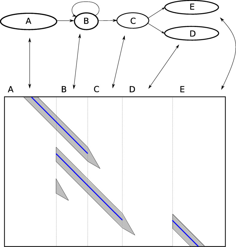
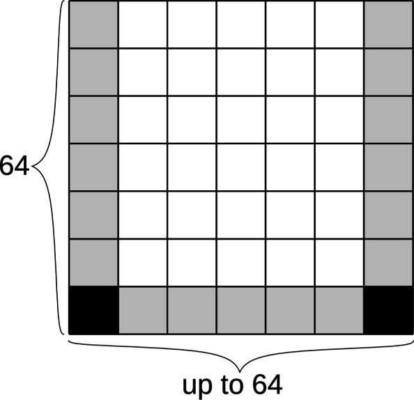
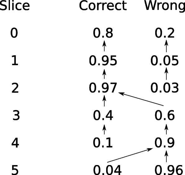
Verification
Claims the paper makes
The claims and statistics of this paper haven’t been checked yet.
Run the check — free, no account needed. It reads the open-access text and checks the sources it cites.
Claims other papers make about this one
Each is checked against this paper’s own text: does it say what the citing paper says it does?
The cited source doesn’t support the claim as written.
In the citing paper
“After extension, paths are scored based on the alignment's quality, and the best-scoring path is selected as the optimal alignment.”
From Whole-Genome Alignment: Methods, Challenges, and Future Directions (2024) · cites this paper as [50]
Checked by a reasoning model — may be wrong.
Experimental — accuracy not yet measuredThe source backs part of the claim, not all of it — or backs it for a different population, condition or comparison.
In the citing paper
“The reference genome is first constructed into a graph where nodes represent sequence blocks and edges represent possible transitions between these blocks.”
From Whole-Genome Alignment: Methods, Challenges, and Future Directions (2024) · cites this paper as [50]
Experimental — accuracy not yet measuredThe source backs part of the claim, not all of it — or backs it for a different population, condition or comparison.
In the citing paper
“GraphAligner is specifically adept at handling complex graph structures with varying paths, such as those introduced by repeats or structural variants, which are often challenging for linear alignment methods.”
From Whole-Genome Alignment: Methods, Challenges, and Future Directions (2024) · cites this paper as [50]
Experimental — accuracy not yet measuredThe source backs part of the claim, not all of it — or backs it for a different population, condition or comparison.
In the citing paper
“The algorithm treats the reference genome as a graph where variations and alternative splicing events are represented as branches [50].”
From Whole-Genome Alignment: Methods, Challenges, and Future Directions (2024) · cites this paper as [50]
Experimental — accuracy not yet measuredThe source backs part of the claim, not all of it — or backs it for a different population, condition or comparison.
In the citing paper
“GraphAligner is particularly useful in genomic studies where the reference genome includes significant alternative paths, such as in cancer genomics, where somatic mutations, insertions, deletions, and rearrangements are common, or in research involving highly polymorphic species.”
From Whole-Genome Alignment: Methods, Challenges, and Future Directions (2024) · cites this paper as [50]
Experimental — accuracy not yet measured
The cited source says what the claim attributes to it.
In the citing paper
“GraphAligner is designed to align long reads to a graph-based reference.”
From Whole-Genome Alignment: Methods, Challenges, and Future Directions (2024) · cites this paper as [50]
The cited source says what the claim attributes to it.
In the citing paper
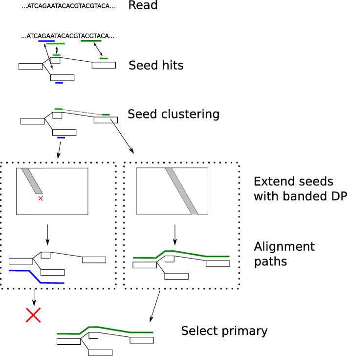
“Using dynamic programming, seeds are extended along the paths of the graph. The extension process respects the graph's topology, exploring different paths where the read might align with segments of the reference;”
From Whole-Genome Alignment: Methods, Challenges, and Future Directions (2024) · cites this paper as [50]
The cited source says what the claim attributes to it.
In the citing paper
“The algorithm begins with identifying seed matches between the read and subsequences in the graph. Seeds are typically exact matches that are used as anchor points for more detailed alignment;”
From Whole-Genome Alignment: Methods, Challenges, and Future Directions (2024) · cites this paper as [50]
The check wasn’t confident either way, so it gives no verdict — never disputed.
In the citing paper
“It typically has a worst-case time complexity of O ( k × n × m ), where k is the number of nodes in the graph, n is the length of the reference sequence, and m is the length of the read sequence.”
From Whole-Genome Alignment: Methods, Challenges, and Future Directions (2024) · cites this paper as [50]
Experimental — accuracy not yet measured
Self-check
Percentages, sums and reported differences re-computed from the paper’s own numbers.
The self-check needs the paper’s full text.
Citations
Cites
Needleman, S. B., & Wunsch, C. D. (1970) · Journal of Molecular Biology · doi:10.1016/0022-2836(70)90057-4 · Cited by 11,288
Wenger, A. M., Peluso, P., Rowell, W. J., Chang, P.-C., Hall, R. J., Concepcion, G. T., Ebler, J., Fungtammasan, A., Kolesnikov, A., Olson, N. D., et al. (2019) · Nature Biotechnology · doi:10.1038/s41587-019-0217-9 · Cited by 1,841
Self-citationMulti-platform discovery of haplotype-resolved structural variation in human genomes
Chaisson, M. J. P., Sanders, A. D., Zhao, X., Malhotra, A., Porubsky, D., Rausch, T., Gardner, E. J., Rodriguez, O. L., Guo, L., Collins, R. L., et al. (2019) · Nature Communications · doi:10.1038/s41467-018-08148-z · Cited by 891
Self-citationReducing storage requirements for biological sequence comparison
Roberts, M., Hayes, W., Hunt, B. R., Mount, S. M., & Yorke, J. A. (2004) · Bioinformatics · doi:10.1093/bioinformatics/bth408 · Cited by 485
The design and construction of reference pangenome graphs with minigraph
Li, H., Feng, X., & Chu, C. (2020) · Genome Biology · doi:10.1186/s13059-020-02168-z · Cited by 455
Human Genome Structural Variation Consortium, Porubsky, D., Ebert, P., Audano, P. A., Vollger, M. R., Harvey, W. T., Marijon, P., Ebler, J., Munson, K. M., Sorensen, M., et al. (2021) · Nature Biotechnology · doi:10.1038/s41587-020-0719-5 · Cited by 203
Self-citation
Research works printed but not linked: 60
- Computational Pan-Genomics Consortium. Computational pan-genomics: status, promises and challenges. Brief Bioinforma. 2016; 19(1):118–35.
- Paten B, Novak AM, Eizenga JM, Garrison E. Genome graphs and the evolution of genome inference. Genome Res. 2017; 27(5):665–76. · DOI · Paper page
- Bankevich A, Nurk S, Antipov D, Gurevich AA, Dvorkin M, Kulikov AS, Lesin VM, Nikolenko SI, Pham S, Prjibelski AD, et al. SPAdes: a new genome assembly algorithm and its applications to single-cell sequencing. J Comput Biol. 2012; 19(5):455–77. · DOI
- Antipov D, Korobeynikov A, McLean JS, Pevzner PA. hybridSPAdes: an algorithm for hybrid assembly of short and long reads. Bioinformatics. 2015; 32(7):1009–15. · DOI
- Wick RR, Judd LM, Gorrie CL, Holt KE. Unicycler: resolving bacterial genome assemblies from short and long sequencing reads. PLoS Comput Biol. 2017; 13(6):1005595. · DOI
- Salmela L, Rivals E. LoRDEC: accurate and efficient long read error correction. Bioinformatics. 2014; 30(24):3506–14. · DOI
- Miclotte G, Heydari M, Demeester P, Rombauts S, Van de Peer Y, Audenaert P, Fostier J. Jabba: hybrid error correction for long sequencing reads. Algorithm Mol Biol. 2016; 11(1):10. · DOI
- Wang JR, Holt J, McMillan L, Jones CD. FMLRC: hybrid long read error correction using an FM-index. BMC Bioinformatics. 2018; 19(1):50. · DOI
- Dolzhenko E, Deshpande V, Schlesinger F, Krusche P, Petrovski R, Chen S, Emig-Agius D, Gross A, Narzisi G, Bowman B, et al.ExpansionHunter: a sequence-graph based tool to analyze variation in short tandem repeat regions. Bioinformatics (Oxford, England). 2019; 35:4754–6. · DOI · Paper page
- Hickey G, Heller D, Monlong J, Sibbesen JA, Siren J, Eizenga J, Dawson E, Garrison E, Novak A, Paten B. Genotyping structural variants in pangenome graphs using the vg toolkit. Genome Biol. 2020; 21:35. https://doi.org/10.1186/s13059-020-1941-7. · DOI · Paper page
- Garg S, Rautiainen M, Novak AM, Garrison E, Durbin R, Marschall T. A graph-based approach to diploid genome assembly. Bioinformatics. 2018; 34(13):105–14. · DOI
- Altschul SF, Gish W, Miller W, Myers EW, Lipman DJ. Basic local alignment search tool. J Mol Biol. 1990; 215(3):403–410. · DOI · Paper page
- Li H. Minimap2: pairwise alignment for nucleotide sequences. Bioinformatics. 2018; 34(18):3094–100. · DOI · Paper page
- Li H, Durbin R. Fast and accurate short read alignment with Burrows–Wheeler Transform. bioinformatics. 2009; 25(14):1754–60. · DOI · Paper page
- Sović I, Šikić M, Wilm A, Fenlon SN, Chen S, Nagarajan N. Fast and sensitive mapping of nanopore sequencing reads with graphmap. Nat Commun. 2016; 7:11307. · DOI
- Garrison E, Sirén J, Novak AM, Hickey G, Eizenga JM, Dawson ET, Jones W, Garg S, Markello C, Lin MF, et al.Variation graph toolkit improves read mapping by representing genetic variation in the reference. Nat Biotechnol. 2018; 46:875–9. · DOI · Paper page
- Navarro G. Improved approximate pattern matching on hypertext. Theor Comput Sci. 2000; 237(1):455–63. · DOI
- Equi M, Grossi R, Tomescu AI, Mäkinen V. On the complexity of exact pattern matching in graphs: determinism and zig-zag matching. arXiv preprint arXiv:1902.03560. 2019. · arXiv
- Lee C, Grasso C, Sharlow MF. Multiple sequence alignment using partial order graphs. Bioinformatics. 2002; 18(3):452–64. · DOI
- Kavya VNS, Tayal K, Srinivasan R, Sivadasan N. Sequence alignment on directed graphs. J Comput Biol. 2019; 26(1):53–67. · DOI
- Limasset A, Cazaux B, Rivals E, Peterlongo P. Read mapping on de bruijn graphs. BMC Bioinformatics. 2016; 17(1):237. · DOI
- Jain C, Zhang H, Gao Y, Aluru S. On the complexity of sequence to graph alignment. bioRxiv. 2019. https://doi.org/10.1101/522912. · DOI
- Rautiainen M, Mäkinen V, Marschall T. Bit-parallel sequence-to-graph alignment. Bioinformatics. 2019. https://doi.org/10.1093/bioinformatics/btz162. · DOI
- Myers G. A fast bit-vector algorithm for approximate string matching based on dynamic programming. J ACM (JACM). 1999; 46(3):395–415. · DOI
- Liu B, Guo H, Brudno M, Wang Y. deBGA: read alignment with de bruijn graph-based seed and extension. Bioinformatics. 2016; 32(21):3224–32. · DOI
- Durbin R. Efficient haplotype matching and storage using the positional Burrows–Wheeler Transform (pbwt). Bioinformatics. 2014; 30(9):1266–72. · DOI
- Sirén J, Välimäki N, Mäkinen V. IEEE/ACM Trans Comput Biol Bioinforma (TCBB). 2014; 11(2):375–88. · DOI
- Sirén J. Indexing variation graphs. In: 2017 Proceedings of the Ninteenth Workshop on Algorithm Engineering and Experiments (ALENEX). Society for Industrial and Applied Mathematics: 2017. p. 13–27. https://doi.org/10.1137/1.9781611974768.2. · DOI
- Sirén J, Garrison E, Novak AM, Paten B, Durbin R. Haplotype-aware graph indexes. arXiv preprint arXiv:1805.03834. 2018. · DOI
- Mokveld T, Linthorst J, Al-Ars Z, Holstege H, Reinders M. CHOP: haplotype-aware path indexing in population graphs. bioRxiv. 2019. https://doi.org/10.1101/305268. · DOI
- Ghaffaari A, Marschall T. Fully-sensitive seed finding in sequence graphs using a hybrid index: 2019. p i81–9. https://doi.org/10.1093/bioinformatics/btz341. · DOI
- Ono Y, Asai K, Hamada M. PBSIM: PacBio reads simulator—toward accurate genome assembly. Bioinformatics. 2013; 29(1):119–21. · DOI
- Clarke L, Fairley S, Zheng-Bradley X, Streeter I, Perry E, Lowy E, Tassé A-M, Flicek P. The international genome sample resource (IGSR): a worldwide collection of genome variation incorporating the 1000 genomes project data. Nucleic Acids Res. 2017; 45(D1):854–9. · DOI
- Porubsky D, Ebert P, Audano PA, Vollger MR, Harvey WT, Munson KM, Sorensen M, Sulovari A, Haukness M, Ghareghani M, Human Genome Structural Variation Consortium, Paten B, Devine SE, Sanders AD, Lee C, Chaisson MJP, Korbel JO, Eichler EE, Marschall T. A fully phased accurate assembly of an individual human genome. bioRxiv. 2019. https://www.biorxiv.org/content/10.1101/855049v1.abstract. · DOI
- Krusche P, Trigg L, Boutros PC, Mason CE, Francisco M, Moore BL, Gonzalez-Porta M, Eberle MA, Tezak Z, Lababidi S, et al. Best practices for benchmarking germline small-variant calls in human genomes. Nat Biotechnol. 2019; 37(5):555–60. · DOI · Paper page
- Lowy-Gallego E, Fairley S, Zheng-Bradley X, Ruffier M, Clarke L, Flicek P, Consortium GP, et al.Variant calling on the grch38 assembly with the data from phase three of the 1000 genomes project. Wellcome Open Res. 2019; 4:50. https://doi.org/10.12688/wellcomeopenres.15126.2. · DOI
- Cleary JG, Braithwaite R, Gaastra K, Hilbush BS, Inglis S, Irvine SA, Jackson A, Littin R, Rathod M, Ware D, et al.Comparing variant call files for performance benchmarking of next-generation sequencing variant calling pipelines. BioRxiv. 2015:023754. https://www.biorxiv.org/content/10.1101/023754v2.abstract. · DOI · Paper page
- Zhang H, Jain C, Aluru S. A comprehensive evaluation of long read error correction methods. bioRxiv. 2019. https://doi.org/10.1101/519330. · DOI
- Song L, Florea L, Langmead B. Lighter: fast and memory-efficient sequencing error correction without counting. Genome Biol. 2014; 15(11):509. · DOI
- Chikhi R, Limasset A, Medvedev P. Compacting de bruijn graphs from sequencing data quickly and in low memory. Bioinformatics. 2016; 32(12):201–208. · DOI
- Holt J, McMillan L. Merging of multi-string BWTs with applications. Bioinformatics. 2014; 30(24):3524–31. · DOI
- Li H. Fast construction of FM-index for long sequence reads. Bioinformatics. 2014; 30(22):3274–5. · DOI
- Li H, Handsaker B, Wysoker A, Fennell T, Ruan J, Homer N, Marth G, Abecasis G, Durbin R. The sequence alignment/map format and samtools. Bioinformatics. 2009; 25(16):2078–9. · DOI · Paper page
- Weirather JL, de Cesare M, Wang Y, Piazza P, Sebastiano V, Wang X-J, Buck D, Au KF. Comprehensive comparison of pacific biosciences and oxford nanopore technologies and their applications to transcriptome analysis. F1000Research. 2017; 6:2078–2079. · DOI · Paper page
- Rautiainen M, Durai DA, Chen Y, Xin L, Low HM, Göke J, Marschall T, Schulz MH. AERON: transcript quantification and gene-fusion detection using long reads. 2020. https://www.biorxiv.org/content/10.1101/2020.01.27.921338v1.abstract. · DOI
- Li H. Minimap and miniasm: fast mapping and de novo assembly for noisy long sequences. Bioinformatics. 2016; 32(14):2103–10. · DOI
- Edmonds J, Johnson EL. Matching: a well-solved class of integer linear programs. In: Combinatorial Optimization—Eureka, You Shrink!. Berlin, Heidelberg: Springer: 2003. p. 27–30. https://doi.org/10.1007/3-540-36478-1_3. · DOI
- Medvedev P, Brudno M. Maximum likelihood genome assembly. J Comput Biol. 2009; 16(8):1101–16. · DOI
- Pevzner PA, Tang H, Waterman MS. An Eulerian path approach to DNA fragment assembly. Proc Natl Acad Sci. 2001; 98(17):9748–53. · DOI · Paper page
- Myers EW. The fragment assembly string graph. Bioinformatics. 2005; 21(suppl_2):79–85. · DOI · Paper page
- Koren S, Walenz BP, Berlin K, Miller JR, Bergman NH, Phillippy AM. Canu: scalable and accurate long-read assembly via adaptive k-mer weighting and repeat separation. Genome Res. 2017; 27:215087. · DOI
- Limasset A, Rizk G, Chikhi R, Peterlongo P. Fast and scalable minimal perfect hashing for massive key sets. arXiv preprint arXiv:1702.03154. 2017. · arXiv
- Gog S, Beller T, Moffat A, Petri M. From theory to practice: plug and play with succinct data structures. In: 13th International Symposium on Experimental Algorithms, (SEA 2014): 2014. p. 326–337. · DOI
- Kuosmanen A, Paavilainen T, Gagie T, Chikhi R, Tomescu A, Mäkinen V. Using minimum path cover to boost dynamic programming on dags: co-linear chaining extended. In: International Conference on Research in Computational Molecular Biology. Cham: Springer: 2018. p. 105–21. https://doi.org/10.1007/978-3-319-89929-9_7. · DOI
- Onodera T, Sadakane K, Shibuya T. Detecting superbubbles in assembly graphs. In: International Workshop on Algorithms in Bioinformatics. Berlin, Heidelberg: Springer: 2013. p. 338–48. https://doi.org/10.1007/978-3-642-40453-5_26. · DOI
- Ukkonen E. Algorithms for approximate string matching. Inf Control. 1985; 64(1-3):100–18. · DOI
- Chao K-M, Pearson WR, Miller W. Aligning two sequences within a specified diagonal band. Bioinformatics. 1992; 8(5):481–7. · DOI
- Suzuki H, Kasahara M. Acceleration of nucleotide semi-global alignment with adaptive banded dynamic programming. BioRxiv. 2017:130633. https://www.biorxiv.org/content/10.1101/130633v2.abstract. · DOI
- Zhang Z, Berman P, Wiehe T, Miller W. Post-processing long pairwise alignments. Bioinformatics. 1999; 15(12):1012–9. · DOI
- Viterbi A. Error bounds for convolutional codes and an asymptotically optimum decoding algorithm. IEEE Trans Inf Theory. 1967; 13(2):260–9. · DOI
Cited by
Sorted by citations
The complete sequence of a human genome
Nurk, S., Koren, S., Rhie, A., Rautiainen, M., Bzikadze, A. V., Mikheenko, A., Vollger, M. R., Altemose, N., Uralsky, L., Gershman, A., et al. (2022) · Science · doi:10.1126/science.abj6987 · Cited by 3,136
Self-citationA draft human pangenome reference.
Liao, W.-W., Asri, M., Ebler, J., Doerr, D., Haukness, M., Hickey, G., Lu, S., Lucas, J. K., Monlong, J., Abel, H. J., et al. (2023) · Nature · doi:10.1038/s41586-023-05896-x · Cited by 1,129
Self-citationThe Human Pangenome Project: a global resource to map genomic diversity
Wang, T., Antonacci-Fulton, L., Howe, K., Lawson, H. A., Lucas, J. K., Phillippy, A. M., Popejoy, A. B., Asri, M., Carson, C., Chaisson, M. J. P., et al. (2022) · Nature · doi:10.1038/s41586-022-04601-8 · Cited by 494
Self-citationThe design and construction of reference pangenome graphs with minigraph
Li, H., Feng, X., & Chu, C. (2020) · Genome Biology · doi:10.1186/s13059-020-02168-z · Cited by 455
Pangenomics enables genotyping of known structural variants in 5202 diverse genomes
Sirén, J., Monlong, J., Chang, X., Novak, A. M., Eizenga, J. M., Markello, C., Sibbesen, J. A., Hickey, G., Chang, P.-C., Carroll, A., et al. (2021) · Science · doi:10.1126/science.abg8871 · Cited by 400
Metadata
- Authors
- Rautiainen, M., & Marschall, T.
- Affiliations
- Max Planck Institute for Informatics (DE)
- Corresponding author
- Marschall, Tobias
- Venue
- Genome Biology
- Published
- 2020-09-24
- Volume
- 21
- Issue
- 1
- Pages
- 253-253
- ISSN
- 1465-6906 (ISSN-L)
- 1474-760X
- PMC
- PMC7513500
- OpenAlex
- W3088400220
- Cited by
- 242
- References
- 6
- Citations by year
- 2026: 39 · 2025: 50 · 2024: 53 · 2023: 48 · 2022: 23 · 2021: 19 · 2020: 10
- FWCI
- 8.73
- Type
- journal article
- Language
- en
- Open access
- gold
- doi.org
- Locations
- Genome biology (publishedVersion, cc-by)
- bioRxiv (Cold Spring Harbor Laboratory) (acceptedVersion, cc-by-nd)
- PubMed Central (publishedVersion, cc-by)
- PubMed (publishedVersion)
- DOAJ (DOAJ: Directory of Open Access Journals) (submittedVersion, cc-by-sa)
- MPG.PuRe (Max Planck Society) (submittedVersion, other-oa)
- Funders
- International Max Planck Research School for Environmental, Cellular and Molecular Microbiology
- International Max Planck Research School for Advanced Methods in Process and Systems Engineering
- Topics
- Life Sciences › Biochemistry, Genetics and Molecular Biology › Molecular Biology › Genomics and Phylogenetic Studies
- Physical Sciences › Mathematics › Theoretical Computer Science › Algorithms and Data Compression
- Life Sciences › Biochemistry, Genetics and Molecular Biology › Molecular Biology › Fractal and DNA sequence analysis
- Keywords
- genome graphs, long-read alignment, pangenome graphs, error correction, genome assembly, variant genotyping, genetic variation
- MeSH terms
- Algorithms, Animals, Humans, Software, Sequence Alignment, Genomics
About these checks
Registry, retraction, Cites and statistics results are computed, not judged, with one exception: a printed reference that no index lists is read once by a model before it counts as a citation error. Claims are extracted by a model and kept only when their quote appears verbatim in the text; each cited source is then checked, with a model’s help, for whether it says what the claim relies on. Those verdicts can be wrong — read the claim’s quote and the cited source before relying on one.
Statistics and arithmetic are recomputed, not judged.
Confidence bands are shown only for fields calibrated on our annotated test set. None is calibrated yet, so no band is shown.
What counts as a claim ›How we measure confidence ›How we check this ›
Are you an author, or do you see a problem with this page? Request a review
