

The DOI matches its Crossref record; 142 of the 150 references it cites were found in a registry or an index; 59 of the 67 sources its claims cite were checked for support.
A draft human pangenome reference.
Open accessPublished version of a preprint
Abstract
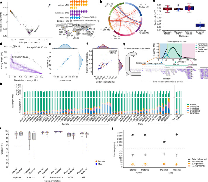
Here the Human Pangenome Reference Consortium presents a first draft of the human pangenome reference. The pangenome contains 47 phased, diploid assemblies from a cohort of genetically diverse individuals. These assemblies cover more than 99% of the expected sequence in each genome and are more than 99% accurate at the structural and base pair levels.
Overview
CoChat Summary
TL;DR
The paper presents a first draft human pangenome reference built from 47 phased, diploid assemblies from genetically diverse individuals, plus graph-based representations and annotations. The draft pangenome improves downstream analyses versus GRCh38, including reducing small-variant discovery errors by 34% and increasing detected structural variants per haplotype by 104%.
Key findings
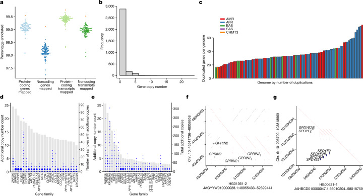
- The draft pangenome was built from 47 phased, diploid assemblies and adds 119 million base pairs of euchromatic polymorphic sequence plus 1,115 gene duplications relative to GRCh38; about 90 million of the added bases came from structural variation.
- Assemblies were reported as >99% complete and >99% accurate at structural and base-pair levels; the assembly reliability pipeline marked only 0.88% (26.4 Mb) of each assembly as unreliable.
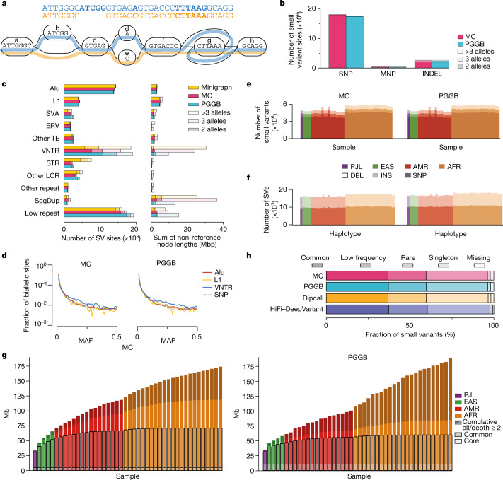
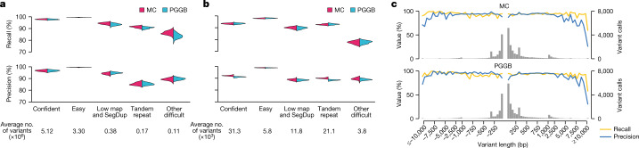
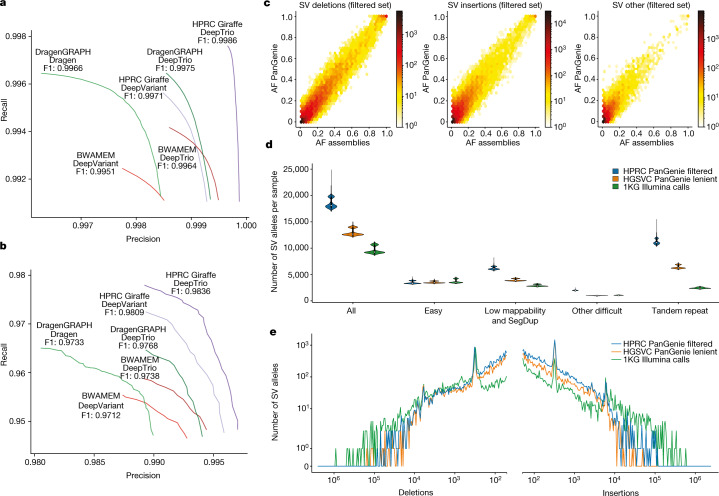
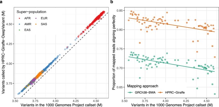
- In short-read analysis, the pangenome workflow reduced small-variant discovery errors by 34% and increased the number of structural variants detected per haplotype by 104% compared with GRCh38-based workflows.
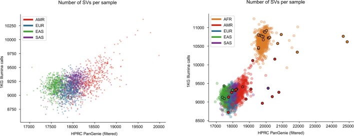
- For 1KG short-read genotyping, the pangenome-based call set gave on average 64,000 more small variants per sample than the 1KG catalogue; for SV genotyping it produced 18,483 SVs per sample versus 9,596 in the short-read 1KG call set.
Methods
- The study assembled 47 fully phased diploid genomes from globally diverse individuals, using PacBio HiFi, Oxford Nanopore, Hi-C, Bionano, and parental Illumina data; assemblies were phased with Trio-Hifiasm and manually/automatically curated.
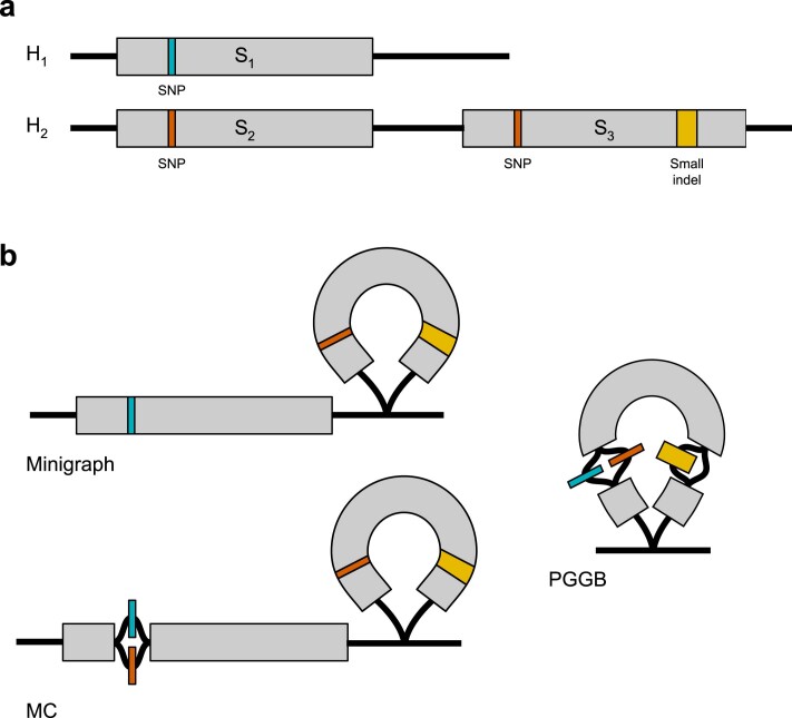
- The authors constructed pangenomes with three graph approaches: Minigraph, Minigraph-Cactus (MC), and PGGB, then evaluated variant representation, graph support, and downstream utility.
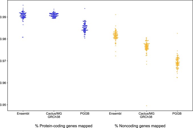
- They benchmarked pangenome-based analyses against GRCh38-based workflows using GIAB, 1KG short reads, and assembly-based comparisons for small variants, SVs, gene annotations, RNA-seq, ChIP-seq/ATAC-seq, VNTRs, and population analyses.
Limitations
- The paper states the cohort is relatively small and that the assembly reliability analysis found roughly an order of magnitude more erroneously assembled sequences in the HPRC assemblies than in T2T-CHM13.
- It explicitly notes remaining issues in highly repetitive regions and complex loci, where variant calling performance was lower and further work is needed; this is a stated limitation.
- The text also makes evident that some analyses are constrained by reference gaps, alignment ambiguity, and incomplete benchmarking truth sets; this is the paper’s implication, stated in the discussion around repetitive regions and underestimation of errors.
Model-written summary. Check it against the paper before relying on it.
Integrity signals
Registry
Cites
Statistics
Figures

Verification
Claims the paper makes
38 Valid · 5 Not valid · 2 Not checked · 206 Own results and interpretations
At least one cited source doesn’t support this claim or points to a different paper, and none confirmed it — see the verdicts below.
In the paper
“The pangenome contains 47 phased, diploid assemblies from a cohort of genetically diverse individuals1.”
§ A draft human pangenome reference > Abstract
What the sources say
- Disputedcites [1] 1000 Genomes Project Consortium. A global reference for human genetic variation. Nature 526, 68–74 (2015). sourceExperimental — accuracy not yet measured
The Abstract (page unavailable) describes a 1000 Genomes resource based on 2,504 individuals from 26 populations, with variants phased onto haplotypes. The Data set overview describes phasing variant sites, not a pangenome containing 47 phased, diploid assemblies. (LLM, conf=0.86)
Checked by a reasoning model — may be wrong.
plain- Asserted: passes — The authors put it forward as true.
- Checkable: passes — It can be checked against evidence.
- Load-bearing: passes — The paper’s conclusions depend on it.
- Based: passes — The paper gives a reason why it holds.
- Rests on an assumption not shown here.
- Disputed
The cited sources support only part of this claim — read each source’s verdict below.
In the paper
“Previous studies have identified tens of megabases of sequence contained within structural variants (SVs) that are polymorphic within the population5.”
§ A draft human pangenome reference > Main
What the sources say
- Partly supportedcites [5] Ebert, P. et al. Haplotype-resolved diverse human genomes and integrated analysis of structural variation. Science 372, eabf7117 (2021). sourceExperimental — accuracy not yet measured
The Results sections on structural variant distribution and complex structural variation document SVs and distinct structural haplotypes in human populations. But the reported ~279 Mbp is the genomic span of SV hotspots, not the amount of sequence contained within polymorphic SVs; the passages do not establish the claimed tens-of-megabases total. (LLM, conf=0.82)
plain- Asserted: passes — The authors put it forward as true.
- Checkable: passes — It can be checked against evidence.
- Load-bearing: passes — The paper’s conclusions depend on it.
- Based: passes — The paper gives a reason why it holds.
- Partly supported
Every source the paper cites for this claim was checked and supports it.
In the paper
“Recently, the Telomere-to-Telomere (T2T) consortium finished the first complete sequence of a haploid human genome, T2T-CHM13, which provides a contiguous representation of each autosome and of chromosome X, with the exception of some ribosomal DNA arrays that remain to be fully resolved3.”
§ A draft human pangenome reference > Main
What the sources say
- Supportedcites [3] Nurk, S. et al. The complete sequence of a human genome. Science 376, 44–53 (2022). source
“A truly complete genome” states that T2T-CHM13 has gapless telomere-to-telomere assemblies for all 22 autosomes and chromosome X. “rDNA assembly” explains that the ordering of repeats in three rDNA arrays could not be fully resolved, so those arrays are represented by model sequences. (LLM, conf=0.93)
plainSingle case- Asserted: passes — The authors put it forward as true.
- Checkable: passes — It can be checked against evidence.
- Load-bearing: passes — The paper’s conclusions depend on it.
- Based: passes — The paper gives a reason why it holds.
- Supported
The cited sources support only part of this claim — read each source’s verdict below.
In the paper
“despite individual SVs being more likely to affect gene function than either individual SNPs or short insertions and deletions (indels)9,10.”
§ A draft human pangenome reference > Main
What the sources say
- Partly supportedcites [9] Chiang, C. et al. The impact of structural variation on human gene expression. Nat. Genet. 49, 692–699 (2017). sourceExperimental — accuracy not yet measured
The Results (Fine-mapping causal variants) state that, per variant, an SV is 28–54 times more likely to modulate gene expression than an SNV or indel. That supports the comparison for gene expression, but the cited analysis does not establish the broader claim about gene function generally. (LLM, conf=0.86)
- Partly supportedcites [10] Sudmant, P. H. et al. An integrated map of structural variation in 2,504 human genomes. Nature 526, 75–81 (2015). sourceExperimental — accuracy not yet measured
The Functional impact of SVs section reports that SV classes were enriched for expression-associated variants relative to the number tested, supporting a greater per-variant effect on gene expression. It uses eQTL associations as a surrogate for functional impact and groups SNPs with indels in the comparison; it does not establish the broader claim about gene function separately against each variant type. (LLM, conf=0.82)
hedgedstates an association- Asserted: passes — The authors put it forward as true.
- Checkable: passes — It can be checked against evidence.
- Load-bearing: passes — The paper’s conclusions depend on it.
- Based: passes — The paper gives a reason why it holds.
- Partly supported
Every source the paper cites for this claim was checked and supports it.
In the paper
“For the core assembler, we chose Trio-Hifiasm20 after detailed benchmarking of several alternatives21.”
§ A draft human pangenome reference > Assembling 47 diverse human genomes
What the sources say
- Supportedcites [20] Cheng, H., Concepcion, G. T., Feng, X., Zhang, H. & Li, H. Haplotype-resolved de novo assembly using phased assembly graphs with hifiasm. Nat. Methods 18, 170–175 (2021). source
Citation 20 identifies Trio-Hifiasm as the assembler the citing authors chose. The Results section (‘Overview of the hifiasm algorithm’) describes hifiasm’s graph-based trio binning, supporting that identification. The separate benchmarking claim is attached to citation 21, not this source. (LLM, conf=0.93)
- Supportedcites [21] Jarvis, E. D. et al. Semi-automated assembly of high-quality diploid human reference genomes. Nature 611, 519–531 (2022). source
The cited paper’s ‘Trios and higher phasing accuracy’ section compares several assembly algorithms and data types. Its ‘Graph phasing is more complete and accurate’ section reports that Trio hifiasm had the strongest combination of quality metrics among the diploid assemblies. The citing authors’ choice of core assembler is their own decision; this source supports the benchmarking offered as its rationale. Page numbers were not available in our copy. (LLM, conf=0.91)
plain- Asserted: passes — The authors put it forward as true.
- Checkable: passes — It can be checked against evidence.
- Load-bearing: unclear — It is unclear whether the paper’s conclusions depend on it.
- Based: passes — The paper gives a reason why it holds.
- Supported
135 more claims · 15 with their cited sources checked
Create a free account to see all 251 claims and every source verdict.
- It may state two separate claims as one. 80
- Probably not a substantial claim. 40
- The quote only partly states this claim. 1
Claims other papers make about this one
Each is checked against this paper’s own text: does it say what the citing paper says it does?
The cited source doesn’t support the claim as written.
In the citing paper
“In addition, the DRAGEN multigenome mapper is already incorporated for SV and CNV calling, something that is not currently possible with any other graph genome implementations because they focus primarily on genotyping variants14,73.”
From Comprehensive genome analysis and variant detection at scale using DRAGEN (2025) · cites this paper as [73]
Checked by a reasoning model — may be wrong.
Experimental — accuracy not yet measuredThe source backs part of the claim, not all of it — or backs it for a different population, condition or comparison.
In the citing paper
“Other biases, for example, in terms of sex, specific diseases, or human ancestral populations could also reduce the impact of AIVC models.115”
From How to build the virtual cell with artificial intelligence: Priorities and opportunities (2024) · cites this paper as [115]
Experimental — accuracy not yet measuredThe source backs part of the claim, not all of it — or backs it for a different population, condition or comparison.
In the citing paper
“For example, population-specific genes may provide insights into local adaptation, while structural variants may contribute to disease susceptibility or resistance in ways that were previously invisible to reference-based analyses [112,113].”
From Origin and Evolution of Genes in Eukaryotes: Mechanisms, Dynamics, and Functional Implications (2025) · cites this paper as [113]
Experimental — accuracy not yet measuredThe source backs part of the claim, not all of it — or backs it for a different population, condition or comparison.
In the citing paper
“These values were chosen after empirical experimentation specifically to filter out spurious mappings as determined by VCF-based comparison with Hi-Fi-based DeepVariant calls 25 .”
From Pangenome graph construction from genome alignments with Minigraph-Cactus (2024) · cites this paper as [25]
Experimental — accuracy not yet measuredThe cited source says what the claim attributes to it.
In the citing paper
“Notably, the first draft of a human pangenome reference has been released by the Human Pangenome Reference Consortium just last year as of the time of writing [19].”
From <tt>SAFARI</tt> : pangenome alignment of ancient DNA using purine/pyrimidine encodings (2025) · cites this paper as [19]
1 more claim about this paper
Create a free account to see every claim other papers make about this one.
Citations
Cites
The Sequence Alignment/Map format and SAMtools
Li, H., Handsaker, B., Wysoker, A., Fennell, T., Ruan, J., Homer, N., Marth, G., Abecasis, G., Durbin, R., & 1000 Genome Project Data Processing Subgroup (2009) · Bioinformatics · doi:10.1093/bioinformatics/btp352 · Cited by 62,041 · cited 1×
“3.1), (Li et al., 2009).”
InfluentialFast gapped-read alignment with Bowtie 2
Langmead, B., & Salzberg, S. L. (2012) · Nature Methods · doi:10.1038/nmeth.1923 · Cited by 56,400
STAR: ultrafast universal RNA-seq aligner
Dobin, A., Davis, C. A., Schlesinger, F., Drenkow, J., Zaleski, C., Jha, S., Batut, P., Chaisson, M., & Gingeras, T. R. (2013) · Bioinformatics · doi:10.1093/bioinformatics/bts635 · Cited by 51,709
BEDTools: a flexible suite of utilities for comparing genomic features
Quinlan, A. R., & Hall, I. M. (2010) · Bioinformatics · doi:10.1093/bioinformatics/btq033 · Cited by 27,437
Initial sequencing and analysis of the human genome
International Human Genome Sequencing Consortium, Whitehead Institute for Biomedical Research, C. F. G. R., Lander, E. S., Linton, L. M., Birren, B., Nusbaum, C., Zody, M. C., Baldwin, J., Devon, K., Dewar, K., et al. (2001) · Nature · doi:10.1038/35057062 · Cited by 24,216
Self-citationRSEM: accurate transcript quantification from RNA-Seq data with or without a reference genome
Li, B., & Dewey, C. N. (2011) · BMC Bioinformatics · doi:10.1186/1471-2105-12-323 · Cited by 22,179
A global reference for human genetic variation
The 1000 Genomes Project Consortium, authors, C., Auton, A., Abecasis, G. R., Steering committee, Altshuler, D. M., Durbin, R. M., Abecasis, G. R., Bentley, D. R., Chakravarti, A., et al. (2015) · Nature · doi:10.1038/nature15393 · Cited by 18,247
Self-citationAn integrated encyclopedia of DNA elements in the human genome
The ENCODE Project Consortium (2012) · Nature · doi:10.1038/nature11247 · Cited by 18,072
Self-citationTwelve years of SAMtools and BCFtools
Danecek, P., Bonfield, J., Liddle, J., Marshall, J., Ohan, V., Pollard, M., Whitwham, A., Keane, T., McCarthy, S., Davies, R. M., et al. (2021) · GigaScience · doi:10.1093/gigascience/giab008 · Cited by 16,449 · cited 2×
“9 was used for filtering the variant sets (Danecek et al., 2021).”
MethodSelf-citationMinimap2: Pairwise alignment for nucleotide sequences
Li, H. (2018) · Bioinformatics · doi:10.1093/bioinformatics/bty191 · Cited by 14,807 · cited 8×
“The sequences of these anchors were them mapped against the target genome with minimap2 (Li, 2018b) using the following command:”
MethodInfluentialSelf-citation
Cited by
Martin, F. J., Amode, M. R., Aneja, A., Austine-Orimoloye, O., Azov, A. G., Barnes, I., Becker, A., Bennett, R., Berry, A. E., Bhai, J. N. N. T., et al. (2022) · Nucleic Acids Research · doi:10.1093/nar/gkac958 · Cited by 1,051
“We have released initial annotation sets for each of these genomes through our Rapid Release site and built a dedicated HPRC project page (https://projects.ensembl. org/hprc).”
BackgroundMethodInfluentialSelf-citationDyer, S. C., Austine-Orimoloye, O., Azov, A. G., Barba, M., Barnes, I., Enriquez, V. P. B., Becker, A., Bennett, R., Beracochea, M., Berry, A. E., et al. (2024) · Nucleic Acids Research · doi:10.1093/nar/gkae1071 · Cited by 859
Self-citationGENCODE: reference annotation for the human and mouse genomes in 2023
Frankish, A., Sala, S. C., Diekhans, M., Jungreis, I., Loveland, J. E., Mudge, J. M., Sisu, C., Wright, J. C., Arnan, C., Barnes, I., et al. (2022) · Nucleic Acids Research · doi:10.1093/nar/gkac1071 · Cited by 706
“We have provided one gene annotation set using CAT with GENCODE as the reference gene set and assisted in the creation of a second GENCODE-derived annotation set by Ensembl (11).”
BackgroundMethodSelf-citationThe complete sequence of a human Y chromosome
Rhie, A., Nurk, S., Cechova, M., Hoyt, S. J., Taylor, D. J., Altemose, N., Hook, P. W., Koren, S., Rautiainen, M., Alexandrov, I. A., et al. (2023) · Nature · doi:10.1038/s41586-023-06457-y · Cited by 471
“The chain files used were created from the GRCh38-based HAL file, downloaded from the cactus-minigraph alignment of Liao et al.(73) The resulting variant-call formats were annotated with predicted molecular consequence and transcript-specific variant deleteriousness scores from PolyPhen-2 and SIFT using Ensembl Varian…”
MethodSelf-citationSchubach, M., Maass, T., Nazaretyan, L., Röner, S., & Kircher, M. (2024) · Nucleic Acids Research · doi:10.1093/nar/gkad989 · Cited by 455
Metadata
- Authors
- Liao, W.-W., Asri, M., Ebler, J., Doerr, D., Haukness, M., Hickey, G., Lu, S., Lucas, J. K., Monlong, J., Abel, H. J., Buonaiuto, S., Chang, X. H., Cheng, H., Chu, J., Colonna, V., Eizenga, J. M., Feng, X., Fischer, C., Fulton, R. S., Garg, S., Groza, C., Guarracino, A., Harvey, W. T., Heumos, S., Howe, K., Jain, M., Lu, T.-Y., Markello, C., Martin, F. J., Mitchell, M. W., Munson, K. M., Mwaniki, M. N., Novak, A. M., Olsen, H. E., Pesout, T., Porubsky, D., Prins, P., Sibbesen, J. A., Sirén, J., Tomlinson, C., Villani, F., Vollger, M. R., Antonacci-Fulton, L. L., Baid, G., Baker, C. A., Belyaeva, A., Billis, K., Carroll, A., Chang, P.-C., Cody, S., Cook, D. E., Cook-Deegan, R. M., Cornejo, O. E., Diekhans, M., Ebert, P., Fairley, S., Fedrigo, O., Felsenfeld, A. L., Formenti, G., Frankish, A., Gao, Y., Garrison, N. A., Giron, C. G., Green, R. E., Haggerty, L., Hoekzema, K., Hourlier, T., Ji, H. P., Kenny, E. E., Koenig, B. A., Kolesnikov, A., Korbel, J. O., Kordosky, J., Koren, S., Lee, H., Lewis, A. P., Magalhães, H., Marco-Sola, S., Marijon, P., McCartney, A., McDaniel, J., Mountcastle, J., Nattestad, M., Nurk, S., Olson, N. D., Popejoy, A. B., Puiu, D., Rautiainen, M., Regier, A. A., Rhie, A., Sacco, S., Sanders, A. D., Schneider, V. A., Schultz, B. I., Shafin, K., Smith, M. W., Sofia, H. J., Abou Tayoun, A. N., Thibaud-Nissen, F., Tricomi, F. F., Wagner, J., Walenz, B., Wood, J. M. D., Zimin, A. V., Bourque, G., Chaisson, M. J. P., Flicek, P., Phillippy, A. M., Zook, J. M., Eichler, E. E., Haussler, D., Wang, T., Jarvis, E. D., Miga, K. H., Garrison, E., Marschall, T., Hall, I. M., Li, H., & Paten, B.
- Affiliations
- Washington University in St. Louis (US)
- University of California, Santa Cruz (US)
- Heinrich Heine University Düsseldorf (DE)
- Yale University (US)
- Institute of Genetics and Biophysics (IT)
- Harvard University (US)
- Dana-Farber Cancer Institute (US)
- University of Tennessee Health Science Center (US)
- Novo Nordisk Foundation (DK)
- McGill University (CA)
- University of Washington (US)
- Quantitative Biology Center (DE)
- Wellcome Sanger Institute (GB)
- Northeastern University (US)
- University of Southern California (US)
- European Bioinformatics Institute (GB)
- Coriell Institute For Medical Research (US)
- University of Pisa (IT)
- University of Copenhagen (DK)
- Google (United States) (US)
- Washington Center (US)
- Rockefeller University (US)
- National Institutes of Health (US)
- Children's Hospital of Philadelphia (US)
- University of California, Los Angeles (US)
- Stanford Medicine (US)
- Icahn School of Medicine at Mount Sinai (US)
- University of California, San Francisco (US)
- National Institute of Standards and Technology (US)
- University of California, Davis (US)
- Johns Hopkins University (US)
- Max Delbrück Center (DE)
- Kyoto University (JP)
- Howard Hughes Medical Institute (US)
- Corresponding author
- Garrison, Erik
- Marschall, Tobias
- Hall, Ira M.
- Li, Heng
- Paten, Benedict
- ORCID
- Liao, Wen-Wei
- Asri, Mobin
- Ebler, Jana
- Doerr, Daniel
- Haukness, Marina
- Hickey, Glenn
- Lu, Shuangjia
- Lucas, Julian K.
- Monlong, Jean
- Abel, Haley J.
- Buonaiuto, Silvia
- Chang, Xian H.
- Cheng, Haoyu
- Chu, Justin
- Colonna, Vincenza
- Eizenga, Jordan M.
- Feng, Xiaowen
- Fulton, Robert S.
- Garg, Shilpa
- Groza, Cristian
- Guarracino, Andrea
- Harvey, William T.
- Heumos, Simon
- Howe, Kerstin
- Jain, Miten
- Lu, Tsung-Yu
- Markello, Charles
- Martin, Fergal J.
- Mitchell, Matthew W.
- Munson, Katherine M.
- Mwaniki, Moses Njagi
- Novak, Adam M.
- Olsen, Hugh E.
- Pesout, Trevor
- Porubsky, David
- Prins, Pjotr
- Sibbesen, Jonas A.
- Sirén, Jouni
- Tomlinson, Chad
- Villani, Flavia
- Vollger, Mitchell R.
- Baid, Gunjan
- Belyaeva, Anastasiya
- Billis, Konstantinos
- Carroll, Andrew
- Chang, Pi-Chuan
- Cook, Daniel E.
- Cook-Deegan, Robert M.
- Cornejo, Omar E.
- Diekhans, Mark
- Ebert, Peter
- Fairley, Susan
- Fedrigo, Olivier
- Formenti, Giulio
- Frankish, Adam
- Gao, Yan
- Garrison, Nanibaa’ A.
- Green, Richard E.
- Haggerty, Leanne
- Hoekzema, Kendra
- Hourlier, Thibaut
- Ji, Hanlee P.
- Kenny, Eimear E.
- Koenig, Barbara A.
- Kolesnikov, Alexey
- Korbel, Jan O.
- Koren, Sergey
- Lee, HoJoon
- Lewis, Alexandra P.
- Magalhães, Hugo
- Marco-Sola, Santiago
- Marijon, Pierre
- McDaniel, Jennifer
- Mountcastle, Jacquelyn
- Nattestad, Maria
- Nurk, Sergey
- Olson, Nathan D.
- Popejoy, Alice B.
- Puiu, Daniela
- Rautiainen, Mikko
- Regier, Allison A.
- Rhie, Arang
- Sacco, Samuel
- Sanders, Ashley D.
- Shafin, Kishwar
- Smith, Michael W.
- Sofia, Heidi J.
- Thibaud-Nissen, Françoise
- Tricomi, Francesca Floriana
- Wagner, Justin
- Walenz, Brian
- Wood, Jonathan M. D.
- Zimin, Aleksey V.
- Bourque, Guillaume
- Chaisson, Mark J. P.
- Flicek, Paul
- Phillippy, Adam M.
- Zook, Justin M.
- Eichler, Evan E.
- Haussler, David
- Wang, Ting
- Jarvis, Erich D.
- Miga, Karen H.
- Garrison, Erik
- Marschall, Tobias
- Hall, Ira M.
- Li, Heng
- Paten, Benedict
- Venue
- Nature
- Published
- 2023-05-10
- Volume
- 617
- Issue
- 7960
- Pages
- 312-324
- ISSN
- 0028-0836 (ISSN-L)
- 1476-4687
- PMC
- PMC10172123
- OpenAlex
- W4376133202
- Cited by
- 1,129
- References
- 150
- Citations by year
- 2026: 300 · 2025: 374 · 2024: 315 · 2023: 132
- FWCI
- 101.10
- Type
- journal article
- Language
- en
- Open access
- hybrid
- doi.org
- Licence
- cc-by
- creativecommons.org/licenses/by/4.0 (tdm)
- creativecommons.org/licenses/by/4.0 (vor)
- Locations
- Nature (publishedVersion, cc-by)
- PubMed Central (publishedVersion, cc-by)
- PubMed (publishedVersion)
- Digital Commons@Becker (Washington University School of Medicine) (submittedVersion, cc-by)
- HAL (submittedVersion)
- Dipòsit Digital de Documents de la UAB (Universitat Autònoma de Barcelona) (submittedVersion, cc-by)
- eScholarship (California Digital Library) (submittedVersion, cc-by)
- UPCommons institutional repository (Universitat Politècnica de Catalunya) (submittedVersion, cc-by-nc-nd)
- Funders
- Wellcome Trust (WT104947/Z/14/Z, WT222155/Z/20/Z, WT108749/Z/15/Z)
- Nederlandse Organisatie voor Wetenschappelijk Onderzoek (2021.040)
- Novo Nordisk Fonden (NNF10CC1016517, NNF21OC0069089)
- National Institutes of Health (OT2OD033761)
- National Human Genome Research Institute (R01HG010485, U24HG009081, U01HG010973, U01HG010963, U01HG010971, U41HG007234, R01HG011274, U01HG010961, R01HG002385, U24HG011853, U24HG007234, R01HG010169, ZIAHG200398, U24HG007497, U24HG010262, U41HG010972, R01HG011649, R01HG006677)
- National Institute of General Medical Sciences (R01GM123489, R35GM130151)
- Topics
- Life Sciences › Biochemistry, Genetics and Molecular Biology › Molecular Biology › Genomics and Phylogenetic Studies
- Life Sciences › Biochemistry, Genetics and Molecular Biology › Genetics › Genomic variations and chromosomal abnormalities
- Life Sciences › Biochemistry, Genetics and Molecular Biology › Genetics › Genetic Associations and Epidemiology
- Keywords
- human pangenome, structural variants, gene duplication, haplotypes, GRCh38, genetic diversity
- MeSH terms
- Alleles, Diploidy, Haplotypes, Humans, Reference Standards, Genetic Variation, Cohort Studies, Genome, Human, Sequence Analysis, DNA, Genomics
About these checks
Registry, retraction, Cites and statistics results are computed, not judged, with one exception: a printed reference that no index lists is read once by a model before it counts as a citation error. Claims are extracted by a model and kept only when their quote appears verbatim in the text; each cited source is then checked, with a model’s help, for whether it says what the claim relies on. Those verdicts can be wrong — read the claim’s quote and the cited source before relying on one.
The claim verdicts this report counts are experimental: their accuracy is not yet measured.
A language model drew the claims from the paper on 2026-10-11, under version 3 of the claim definition (model deepseek-v4.1-flash, prompt extract-v3).
A second model labelled each claim on 2026-10-11 (model jev-1.13-20260917, definition revision gold-guideline-v0.2).
Cited sources are checked with a language model’s help (gpt-6-sol).
Statistics and arithmetic are recomputed, not judged.
Confidence bands are shown only for fields calibrated on our annotated test set. None is calibrated yet, so no band is shown.
What counts as a claim ›How we measure confidence ›How we check this ›
Are you an author, or do you see a problem with this page? Request a review
How to cite
Cite CoChat for the checks on this page, and the paper for its own findings.
- This page
- CoChat. (2026). Citation check: A draft human pangenome reference. https://app.cochat.ai/papers/10.1038/s41586-023-05896-x
- The paper
- Liao, W.-W., Asri, M., Ebler, J., Doerr, D., Haukness, M., Hickey, G., Lu, S., Lucas, J. K., Monlong, J., Abel, H. J., Buonaiuto, S., Chang, X. H., Cheng, H., Chu, J., Colonna, V., Eizenga, J. M., Feng, X., Fischer, C., Fulton, R. S., . . . Paten, B. (2023). A draft human pangenome reference. Nature. https://doi.org/10.1038/s41586-023-05896-x
Data sources
Bibliographic data: Semantic Scholar, OpenAlex, Crossref.
Contains information from the Semantic Scholar Academic Graph Datasets, made available under the ODC Attribution License (ODC-BY 1.0).
Semantic Scholar’s data is described in: Kinney, R., et al. (2023). The Semantic Scholar Open Data Platform. arXiv:2301.10140.
