Student or educator? Sign up with your school email and get 6 months of Pro free.
CoChat

The DOI matches its Crossref record; 121 of the 121 references it cites were found in a registry or an index.

Bayesian Computation Emerges in Generic Cortical Microcircuits through Spike-Timing-Dependent Plasticity

Open access
Nessler, Bernhard, Pfeiffer, Michael, Buesing, Lars, Maass, Wolfgang · 2013 · PLoS Computational Biology

Abstract

The principles by which networks of neurons compute, and how spike-timing dependent plasticity (STDP) of synaptic weights generates and maintains their computational function, are unknown. Preceding work has shown that soft winner-take-all (WTA) circuits, where pyramidal neurons inhibit each other via interneurons, are a common motif of cortical microcircuits. We show through theoretical analysis and computer simulations that Bayesian computation is induced in these network motifs through STDP in combination with activity-dependent changes in the excitability of neurons. The fundamental components of this emergent Bayesian computation are priors that result from adaptation of neuronal excitability and implicit generative models for hidden causes that are created in the synaptic weights through STDP. In fact, a surprising result is that STDP is able to approximate a powerful principle for fitting such implicit generative models to high-dimensional spike inputs: Expectation Maximization. Our results suggest that the experimentally observed spontaneous activity and trial-to-trial variability of cortical neurons are essential features of their information processing capability, since their functional role is to represent probability distributions rather than static neural codes. Furthermore it suggests networks of Bayesian computation modules as a new model for distributed information processing in the cortex.

Overview

The claims and statistics of this paper haven’t been checked yet.

Free: it reads the open-access text and checks the first 5 claims that cite a source we can check. Create a free account to check every claim.

A few free checks a day · papers already verified open instantly · results are public

Integrity signals

Registry

Crossref · 10.1371/journal.pcbi.1003037

Cites

121 of 121 references verified0 citation errors · 0 not checkable

Statistics

Figures

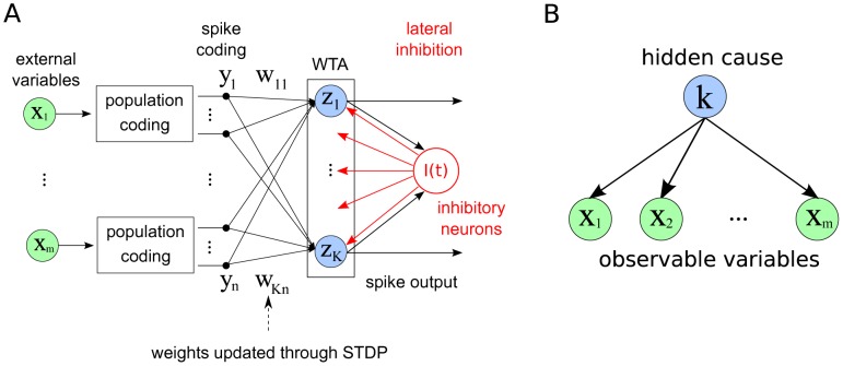
Figure 1 The network model and its probabilistic interpretation. A Circuit architecture. External input variables are encoded by populations of spiking neurons, which feed into a Winner-take-all (WTA) circuit. Neurons within the WTA circuit compete via lateral inhibition and have their input weights updated through STDP. Spikes from the WTA circuit constitute the output of the system. B Generative probabilistic model for a multinomial mixture: A vector of external input variables is dependent on a hidden cause, which is represented by the discrete random variable . In this model it is assumed that the 's are conditionally independent of each other, given . The inference task is to infer the value of , given the observations for . Our neuronal network model encodes the conditional probabilities of the graphical model into the weight vector , such that the activity of the network can be understood as execution of this inference task.
Figure 1 The network model and its probabilistic interpretation. A Circuit architecture. External input variables are encoded by populations of spiking neurons, which feed into a Winner-take-all (WTA) circuit. Neurons within the WTA circuit compete via lateral inhibition and have their input weights updated through STDP. Spikes from the WTA circuit constitute the output of the system. B Generative probabilistic model for a multinomial mixture: A vector of external input variables is dependent on a hidden cause, which is represented by the discrete random variable . In this model it is assumed that the 's are conditionally independent of each other, given . The inference task is to infer the value of , given the observations for . Our neuronal network model encodes the conditional probabilities of the graphical model into the weight vector , such that the activity of the network can be understood as execution of this inference task.CC BY · PubMed Central
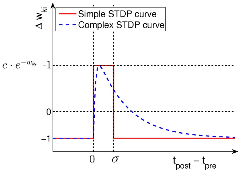
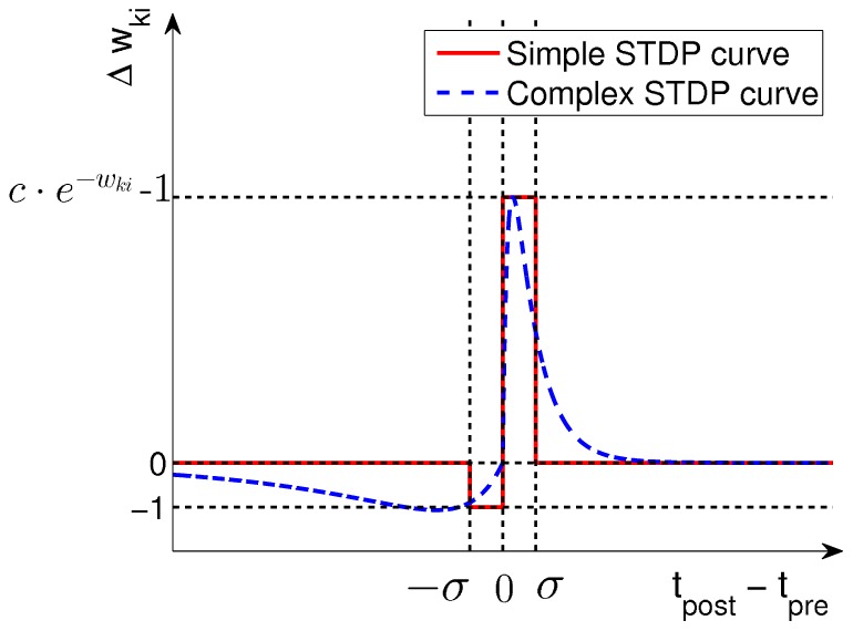
Figure 2 Learning curves for STDP. Under the simple STDP model (red curve), potentiation occurs only if the postsynaptic spike falls within a time window of length (typically ms) after the presynaptic spike. The convergence properties of this simpler version in conjunction with rectangular non-additive EPSPs are easier to analyze. In our simulations we use the more complex version (blue dashed curve) in combination with EPSPs that are modeled as biologically realistic -kernels (with plausible time-constants for rise and decay of respectively ms).
Figure 2 Learning curves for STDP. Under the simple STDP model (red curve), potentiation occurs only if the postsynaptic spike falls within a time window of length (typically ms) after the presynaptic spike. The convergence properties of this simpler version in conjunction with rectangular non-additive EPSPs are easier to analyze. In our simulations we use the more complex version (blue dashed curve) in combination with EPSPs that are modeled as biologically realistic -kernels (with plausible time-constants for rise and decay of respectively ms).CC BY · PubMed Central
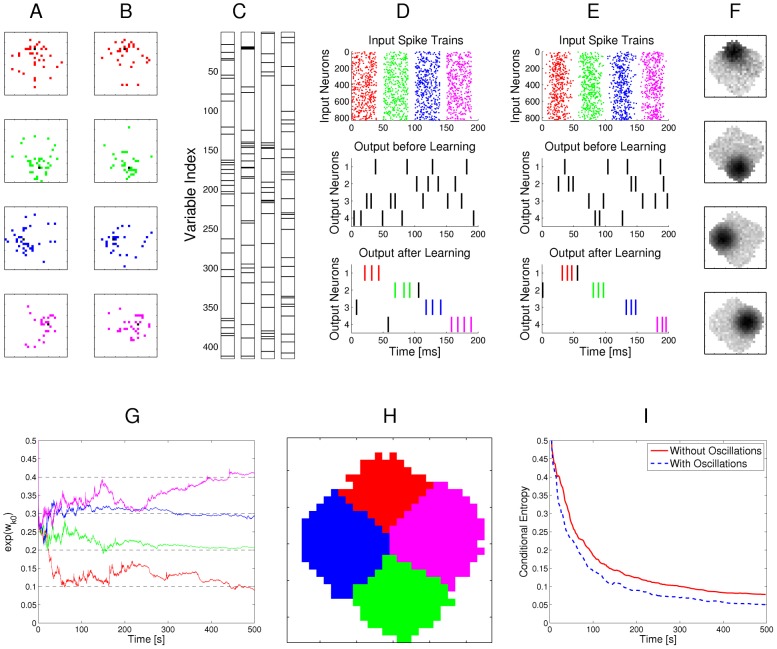
Figure 3 Example for the emergence of Bayesian computation through STDP and adaptation of neural excitability. A, B: Visualization of hidden structure in the spike inputs shown in D, E: Each row in panels A and B shows two results of drawing pixels from the same Gauss distribution over a 28×28 pixel array. Four different Gauss distributions were used in the four rows, and the location of their center represents the latent variable behind the structure of the input spike train. C: Transformation of the four 2D images in B into four linear arrays, resulting from random projections from 2D locations to 1D indices. Black lines indicate active pixels, and pixels that were active in less than 4 of all images were removed before the transformation (these pixels are white in panel H). By the random projection, both the 2D structure of the underlying pixel array and the value of the latent variable are hidden when the binary 1D vector is encoded through population coding into the spike trains that the neural circuit receives. D: Top row: Spike trains from 832 input neurons that result from the four linear patterns shown in panel C (color of spikes indicates which of the four hidden processes had generated the underlying 2D pattern, after 50 ms another 2D pattern is encoded). The middle and bottom row show the spike output of the four output neurons at the beginning and after 500 s of unsupervised learning with continuous spike inputs (every 50 ms another 2D pattern was randomly drawn from one of the 4 different Gauss distributions, with different prior probabilities of 0.1, 0.2, 0.3, and 0.4.). Color of spikes indicates the emergent specialization of the four output neurons on the four hidden processes for input generation. Black spikes indicate incorrect guesses of hidden cause. E: Same as D, but with a superimposed 20 Hz oscillation on the firing rates of input neurons and membrane potentials of the output neurons. Fewer error spikes occur in the output, and output spikes are more precisely timed. F: Internal models (weight vectors ) of output neurons after learning (pixel array). G: Autonomous learning of priors , that takes place simultaneously with the learning of internal models. H: Average “winner” among the four output neurons for a test example (generated with equal probability by any of the 4 Gaussians) when a particular pixel was drawn in this test example, indicating the impact of the learned priors on the output response. I: Emergent discrimination capability of the output neurons during learning (red curve). The dashed blue curve shows that a background oscillation as in E speeds up discrimination learning. Curves in G and I represent averages over 20 repetitions of the learning experiment.
Figure 3 Example for the emergence of Bayesian computation through STDP and adaptation of neural excitability. A, B: Visualization of hidden structure in the spike inputs shown in D, E: Each row in panels A and B shows two results of drawing pixels from the same Gauss distribution over a 28×28 pixel array. Four different Gauss distributions were used in the four rows, and the location of their center represents the latent variable behind the structure of the input spike train. C: Transformation of the four 2D images in B into four linear arrays, resulting from random projections from 2D locations to 1D indices. Black lines indicate active pixels, and pixels that were active in less than 4 of all images were removed before the transformation (these pixels are white in panel H). By the random projection, both the 2D structure of the underlying pixel array and the value of the latent variable are hidden when the binary 1D vector is encoded through population coding into the spike trains that the neural circuit receives. D: Top row: Spike trains from 832 input neurons that result from the four linear patterns shown in panel C (color of spikes indicates which of the four hidden processes had generated the underlying 2D pattern, after 50 ms another 2D pattern is encoded). The middle and bottom row show the spike output of the four output neurons at the beginning and after 500 s of unsupervised learning with continuous spike inputs (every 50 ms another 2D pattern was randomly drawn from one of the 4 different Gauss distributions, with different prior probabilities of 0.1, 0.2, 0.3, and 0.4.). Color of spikes indicates the emergent specialization of the four output neurons on the four hidden processes for input generation. Black spikes indicate incorrect guesses of hidden cause. E: Same as D, but with a superimposed 20 Hz oscillation on the firing rates of input neurons and membrane potentials of the output neurons. Fewer error spikes occur in the output, and output spikes are more precisely timed. F: Internal models (weight vectors ) of output neurons after learning (pixel array). G: Autonomous learning of priors , that takes place simultaneously with the learning of internal models. H: Average “winner” among the four output neurons for a test example (generated with equal probability by any of the 4 Gaussians) when a particular pixel was drawn in this test example, indicating the impact of the learned priors on the output response. I: Emergent discrimination capability of the output neurons during learning (red curve). The dashed blue curve shows that a background oscillation as in E speeds up discrimination learning. Curves in G and I represent averages over 20 repetitions of the learning experiment.CC BY · PubMed Central
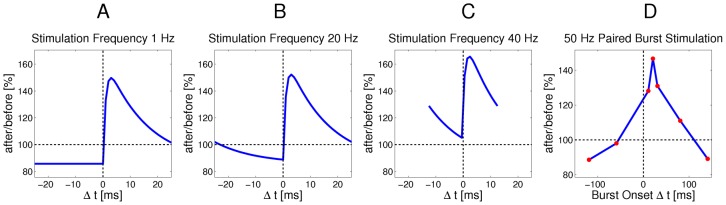
Figure 4 Relationship between the continuous-time SEM model and experimental data on synaptic plasticity. A–C: The effect of the continuous-time plasticity rule in Eq. (18) at a single synapse for different stimulation frequencies and different time-differences between pre- and post-synaptic spike pairs. Only time-intervals without overlapping pairs are shown. A: For very low stimulation frequencies (1 Hz) the standard shape of the complex learning rule from Fig. 2 is recovered. B: At a stimulation frequency of 20 Hz the plasticity curve shifts more towards LTP, and depression is no longer time independent, due to overlapping EPSPs. C: At high stimulation frequencies of 40 Hz or above, the STDP curve shifts towards only LTP, and thus becomes similar to a rate-based Hebbian learning rule. D: Cumulative effect of pre- and post-synaptic burst stimulation (50 Hz bursts of 5 pre-synaptic and 4 post-synaptic spikes) with different onset delays of -120, -60, 10, 20, 30, 80 and 140 ms (time difference between the onsets of the post- and pre-synaptic bursts). As in [55], the amount of overlap between bursts determines the magnitude of LTP, rather than the exact temporal order of spikes.
Figure 4 Relationship between the continuous-time SEM model and experimental data on synaptic plasticity. A–C: The effect of the continuous-time plasticity rule in Eq. (18) at a single synapse for different stimulation frequencies and different time-differences between pre- and post-synaptic spike pairs. Only time-intervals without overlapping pairs are shown. A: For very low stimulation frequencies (1 Hz) the standard shape of the complex learning rule from Fig. 2 is recovered. B: At a stimulation frequency of 20 Hz the plasticity curve shifts more towards LTP, and depression is no longer time independent, due to overlapping EPSPs. C: At high stimulation frequencies of 40 Hz or above, the STDP curve shifts towards only LTP, and thus becomes similar to a rate-based Hebbian learning rule. D: Cumulative effect of pre- and post-synaptic burst stimulation (50 Hz bursts of 5 pre-synaptic and 4 post-synaptic spikes) with different onset delays of -120, -60, 10, 20, 30, 80 and 140 ms (time difference between the onsets of the post- and pre-synaptic bursts). As in [55], the amount of overlap between bursts determines the magnitude of LTP, rather than the exact temporal order of spikes.CC BY · PubMed Central
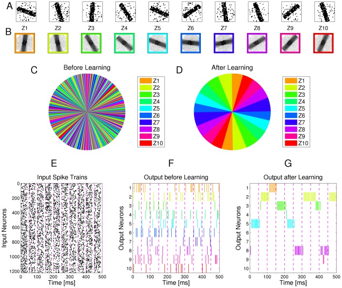
Figure 5 Emergence of orientation selective cells for visual input consisting of oriented bars with random orientations. A Examples of -pixel input images with oriented bars and additional background noise. B Internal models (weight vectors of output neurons ) that are learned through STDP after the presentation of input images (each encoded by spike trains for 50 ms, as in Fig. 3). C, D Plot of the most active neuron for images of bars with orientations from to in steps. Colors correspond to the colors of neurons in B. Before training (C), the output neurons fire without any apparent pattern. After training (D) they specialize on different orientations and cover the range of possible angles approximately uniformly. E: Spike train encoding of the 10 samples in A. F,G: Spike trains produced by the output neurons in response to these samples before and after learning with STDP for 200 s. Colors of the spikes indicate the identity of the output neuron, according to the color code in B.
Figure 5 Emergence of orientation selective cells for visual input consisting of oriented bars with random orientations. A Examples of -pixel input images with oriented bars and additional background noise. B Internal models (weight vectors of output neurons ) that are learned through STDP after the presentation of input images (each encoded by spike trains for 50 ms, as in Fig. 3). C, D Plot of the most active neuron for images of bars with orientations from to in steps. Colors correspond to the colors of neurons in B. Before training (C), the output neurons fire without any apparent pattern. After training (D) they specialize on different orientations and cover the range of possible angles approximately uniformly. E: Spike train encoding of the 10 samples in A. F,G: Spike trains produced by the output neurons in response to these samples before and after learning with STDP for 200 s. Colors of the spikes indicate the identity of the output neuron, according to the color code in B.CC BY · PubMed Central
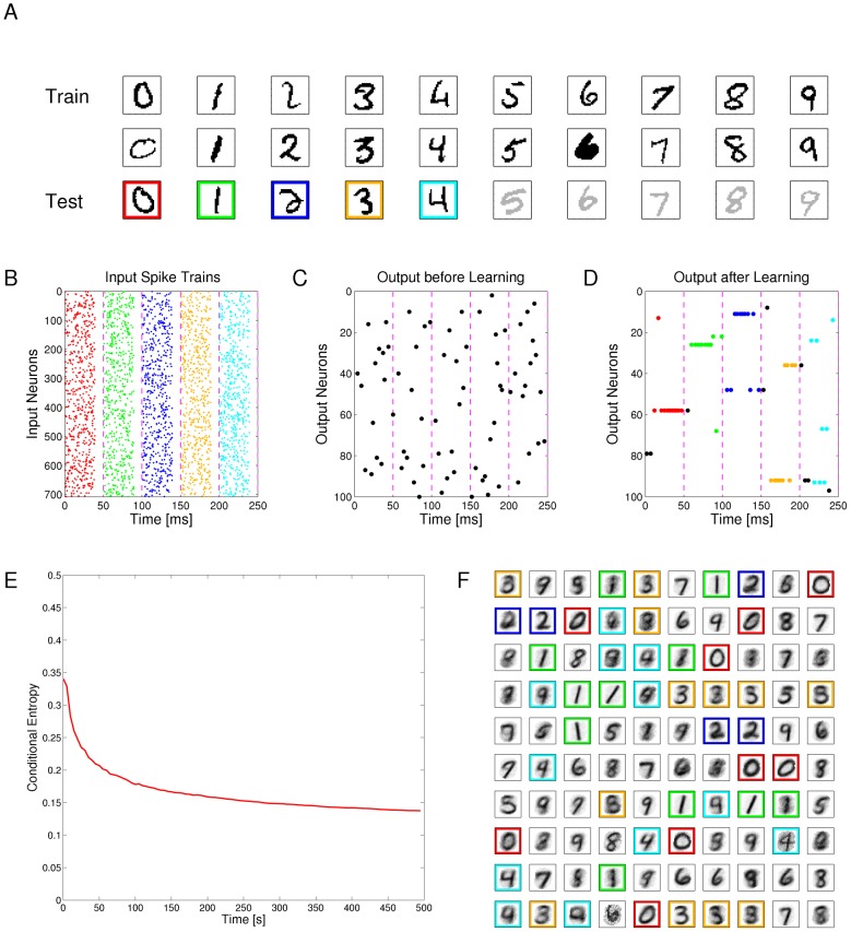
Figure 6 Emergent discrimination of handwritten digits through STDP. A: Examples of digits from the MNIST dataset. The third and fourth row contain test examples that had not been shown during learning via STDP. B: Spike train encoding of the first 5 samples in the third row of A. Colors illustrate the different classes of digits. C, D: Spike trains produced by the output neurons before and after learning with STDP for 500 s. Colored spikes indicate that the class of the input and the class for which the neuron is mostly selective (based on human classification of its generative model shown in F) agree, otherwise spikes are black. E: Temporal evolution of the self-organization process of the 100 output neurons (for the complex version of STDP-curve shown in Fig. 1B), measured by the conditional entropy of digit labels under the learned models at different time points. F: Internal models generated by STDP for the 100 output neurons after 500 s. The network had not received any information about the number of different digits that exist and the colors for different ways of writing the first 5 digits were assigned by the human supervisor. On the basis of this assignment the test samples in row 3 of panel A had been recognized correctly.
Figure 6 Emergent discrimination of handwritten digits through STDP. A: Examples of digits from the MNIST dataset. The third and fourth row contain test examples that had not been shown during learning via STDP. B: Spike train encoding of the first 5 samples in the third row of A. Colors illustrate the different classes of digits. C, D: Spike trains produced by the output neurons before and after learning with STDP for 500 s. Colored spikes indicate that the class of the input and the class for which the neuron is mostly selective (based on human classification of its generative model shown in F) agree, otherwise spikes are black. E: Temporal evolution of the self-organization process of the 100 output neurons (for the complex version of STDP-curve shown in Fig. 1B), measured by the conditional entropy of digit labels under the learned models at different time points. F: Internal models generated by STDP for the 100 output neurons after 500 s. The network had not received any information about the number of different digits that exist and the colors for different ways of writing the first 5 digits were assigned by the human supervisor. On the basis of this assignment the test samples in row 3 of panel A had been recognized correctly.CC BY · PubMed Central
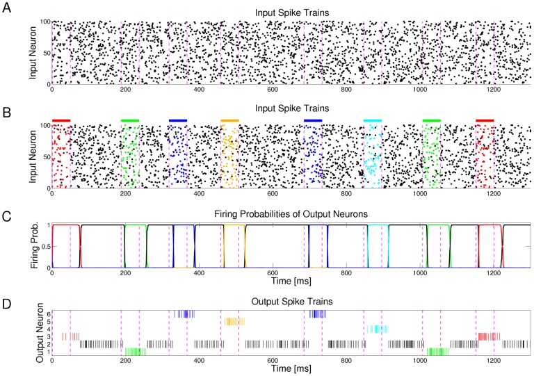
Figure 7 Output neurons self-organize via STDP to detect and represent spatio-temporal spike patterns. A: Sample of the Poisson input spike trains at 20 Hz (only 100 of the 500 input channels are shown). Dashed vertical lines mark time segments of 50 ms length where spatio-temporal spike patterns are embedded into noise. B: Same spike input as in A, but spikes belonging to five repeating spatio-temporal patterns (frozen Poisson spike patterns at 15 Hz) are marked in five different colors. These spike patterns are superimposed by noise (Poisson spike trains at 5 Hz), and interrupted by segments of pure noise of the same statistics (Poisson spike trains at 20 Hz) for intervals of randomly varying time lengths. C, D: Firing probabilities and spike outputs of 6 output neurons (z-neurons in Fig. 1A) for the spike input shown in A, after applying STDP for 200 s to continuous spike trains of the same structure (without any supervision or reward). These 6 output neurons have self-organized so that 5 of them specialize on one of the 5 spatio-temporal patterns. One of the 6 output neurons (firing probability and spikes marked in black) only responds to the noise between these patterns. The spike trains in A represent test inputs, that had never been shown during learning.
Figure 7 Output neurons self-organize via STDP to detect and represent spatio-temporal spike patterns. A: Sample of the Poisson input spike trains at 20 Hz (only 100 of the 500 input channels are shown). Dashed vertical lines mark time segments of 50 ms length where spatio-temporal spike patterns are embedded into noise. B: Same spike input as in A, but spikes belonging to five repeating spatio-temporal patterns (frozen Poisson spike patterns at 15 Hz) are marked in five different colors. These spike patterns are superimposed by noise (Poisson spike trains at 5 Hz), and interrupted by segments of pure noise of the same statistics (Poisson spike trains at 20 Hz) for intervals of randomly varying time lengths. C, D: Firing probabilities and spike outputs of 6 output neurons (z-neurons in Fig. 1A) for the spike input shown in A, after applying STDP for 200 s to continuous spike trains of the same structure (without any supervision or reward). These 6 output neurons have self-organized so that 5 of them specialize on one of the 5 spatio-temporal patterns. One of the 6 output neurons (firing probability and spikes marked in black) only responds to the noise between these patterns. The spike trains in A represent test inputs, that had never been shown during learning.CC BY · PubMed Central
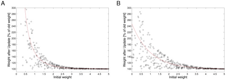
Figure 8 Ideal dependence of weight potentiation under STDP on the initial value of the weight (solid lines). Open circles represent results of samples from this ideal curve with 100% noise, that can be used in the previously discussed computer experiments with almost no loss in performance. A: Dependence of weight potentiation on initial weight according to the STDP rule in Eq. (5). B: Same with an additional factor .
Figure 8 Ideal dependence of weight potentiation under STDP on the initial value of the weight (solid lines). Open circles represent results of samples from this ideal curve with 100% noise, that can be used in the previously discussed computer experiments with almost no loss in performance. A: Dependence of weight potentiation on initial weight according to the STDP rule in Eq. (5). B: Same with an additional factor .CC BY · PubMed Central
Figure 9 STDP learning curves with time-dependent LTD. Under the simple STDP model (red curve), weight-dependent LTP occurs only if the postsynaptic spike falls within a time window of length after the presynaptic spike, and LTD occurs in a time window of the same length, but for the opposite order of spikes. This can be extended to a more complex STDP rule (blue dashed curve), in which both LTP and LTD follow -kernels with different time constants, typically with longer time-constants for LTD.
Figure 9 STDP learning curves with time-dependent LTD. Under the simple STDP model (red curve), weight-dependent LTP occurs only if the postsynaptic spike falls within a time window of length after the presynaptic spike, and LTD occurs in a time window of the same length, but for the opposite order of spikes. This can be extended to a more complex STDP rule (blue dashed curve), in which both LTP and LTD follow -kernels with different time constants, typically with longer time-constants for LTD.CC BY · PubMed Central

Verification

Claims the paper makes

The claims and statistics of this paper haven’t been checked yet.

Free: it reads the open-access text and checks the first 5 claims that cite a source we can check. Create a free account to check every claim.

A few free checks a day · papers already verified open instantly · results are public

Claims other papers make about this one

Each is checked against this paper’s own text: does it say what the citing paper says it does?

Self-check

Percentages, sums and reported differences re-computed from the paper’s own numbers.

The self-check needs the paper’s full text.

Citations

Cites

Show all 121 references

Research works printed but not linked: 2

  1. Bishop CM (2006) Pattern Recognition and Machine Learning. New York: Springer.
  2. G Celeux, 1985, The SEM algorithm: A probabilistic teacher algorithm derived from the EM algorithm for the mixture problem, Comput Statist Quater, 2, 73

Cited by

See all 281

Metadata

Authors
Nessler, B., Pfeiffer, M., Buesing, L., & Maass, W.
Affiliations
  • Graz University of Technology (AT)
  • University of Zurich (CH)
Corresponding author
Nessler, Bernhard
Venue
PLoS Computational Biology
Published
2013-04-25
Volume
9
Issue
4
Pages
e1003037
ISSN
  • 1553-734X (ISSN-L)
  • 1553-7358
OpenAlex
W2003400208
Cited by
281
References
121
Citations by year
2026: 6 · 2025: 11 · 2024: 18 · 2023: 17 · 2022: 16 · 2021: 25 · 2020: 18 · 2019: 21 · 2018: 25 · 2017: 35 · 2016: 37 · 2015: 28 · 2014: 18 · 2013: 5
FWCI
16.02
Type
journal article
Language
en
Open access
Locations
  • PLoS Computational Biology (publishedVersion, cc-by)
  • Europe PMC (PubMed Central) (publishedVersion, cc-by)
  • PubMed Central (publishedVersion, cc-by)
  • PubMed (publishedVersion)
  • Zurich Open Repository and Archive (University of Zurich) (acceptedVersion, cc-by)
  • RePEc: Research Papers in Economics (submittedVersion)
  • DOAJ (DOAJ: Directory of Open Access Journals) (submittedVersion, cc-by-sa)
  • Repository for Publications and Research Data (ETH Zurich) (submittedVersion, cc-by)
  • Zurich Open Repository and Archive (University of Zurich) (submittedVersion, cc-by)
  • ETH Zürich Research Collection (cc-by)
  • Zurich Open Repository and Archive (University of Zurich)
Funders
  • Samsung Advanced Institute of Technology
  • European Commission (269921, 243914, 506778, 216593)
  • Universität Zürich
  • Samsung
Topics
  • Life Sciences › Neuroscience › Cognitive Neuroscience › Neural dynamics and brain function
  • Life Sciences › Neuroscience › Cellular and Molecular Neuroscience › Neuroscience and Neuropharmacology Research
  • Life Sciences › Neuroscience › Cognitive Neuroscience › Memory and Neural Mechanisms
Keywords
Bayesian computation, spike-timing-dependent plasticity, cortical microcircuits, winner-take-all circuit, implicit generative models, expectation-maximization algorithm, spontaneous activity, trial-to-trial variability, distributed information processing, pyramidal neurons, interneurons
MeSH terms
Action Potentials, Animals, Bayes Theorem, Brain, Computer Simulation, Humans, Models, Neurological, Nerve Net, Synaptic Transmission, Neuronal Plasticity, Neurons, Probability, Synapses, Computational Biology

About these checks

Registry, retraction, Cites and statistics results are computed, not judged, with one exception: a printed reference that no index lists is read once by a model before it counts as a citation error. Claims are extracted by a model and kept only when their quote appears verbatim in the text; each cited source is then checked, with a model’s help, for whether it says what the claim relies on. Those verdicts can be wrong — read the claim’s quote and the cited source before relying on one.

Statistics and arithmetic are recomputed, not judged.

Confidence bands are shown only for fields calibrated on our annotated test set. None is calibrated yet, so no band is shown.

What counts as a claim ›How we measure confidence ›How we check this ›

Are you an author, or do you see a problem with this page? Request a review

How to cite

Cite CoChat for the checks on this page, and the paper for its own findings.

This page
CoChat. (2026). Citation check: Bayesian Computation Emerges in Generic Cortical Microcircuits through Spike-Timing-Dependent Plasticity. https://app.cochat.ai/papers/10.1371/journal.pcbi.1003037
The paper
Nessler, B., Pfeiffer, M., Buesing, L., & Maass, W. (2013). Bayesian Computation Emerges in Generic Cortical Microcircuits through Spike-Timing-Dependent Plasticity. PLoS Computational Biology. https://doi.org/10.1371/journal.pcbi.1003037

Data sources

Bibliographic data: Semantic Scholar, OpenAlex, Crossref.

Contains information from the Semantic Scholar Academic Graph Datasets, made available under the ODC Attribution License (ODC-BY 1.0).

Semantic Scholar’s data is described in: Kinney, R., et al. (2023). The Semantic Scholar Open Data Platform. arXiv:2301.10140.