Cited by 302Single-cell and spatial transcriptomicsGene expression and cancer classificationGenomics and Phylogenetic Studies

The DOI matches its Crossref record; 20 of the 20 references it cites were found in a registry or an index.

BASiCS: Bayesian Analysis of Single-Cell Sequencing Data

Open access
Vallejos, Catalina A., Marioni, John C., Richardson, Sylvia·2015·PLOS Computational Biology

Abstract

Single-cell mRNA sequencing can uncover novel cell-to-cell heterogeneity in gene expression levels in seemingly homogeneous populations of cells. However, these experiments are prone to high levels of unexplained technical noise, creating new challenges for identifying genes that show genuine heterogeneous expression within the population of cells under study. BASiCS (Bayesian Analysis of Single-Cell Sequencing data) is an integrated Bayesian hierarchical model where: (i) cell-specific normalisation constants are estimated as part of the model parameters, (ii) technical variability is quantified based on spike-in genes that are artificially introduced to each analysed cell's lysate and (iii) the total variability of the expression counts is decomposed into technical and biological components. BASiCS also provides an intuitive detection criterion for highly (or lowly) variable genes within the population of cells under study. This is formalised by means of tail posterior probabilities associated to high (or low) biological cell-to-cell variance contributions, quantities that can be easily interpreted by users. We demonstrate our method using gene expression measurements from mouse Embryonic Stem Cells. Cross-validation and meaningful enrichment of gene ontology categories within genes classified as highly (or lowly) variable supports the efficacy of our approach.

Overview

The claims and statistics of this paper haven’t been checked yet.

Run the check — free, no account needed. It reads the open-access text and checks the sources it cites.

A few free checks a day · papers already verified open instantly · results are public

Integrity signals

Registry

Crossref · 10.1371/journal.pcbi.1004333

Cites

20 of 20 references verified0 citation errors · 0 not checkable

Statistics

Figures

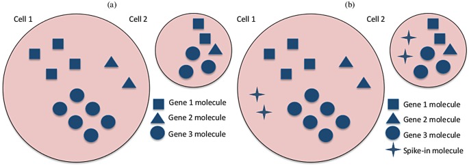
Fig 1 Graphical representation of gene expression in two cells from a homogeneous population but with different total mRNA content. (a) Three biological genes have the same expression rates in both cells, however cell 1 doubles cell 2 in terms of total mRNA content. As a result, the expression counts in cell 1 will be roughly twice as much as those from cell 2, for all genes. In terms of the cell-specific size factors ϕ j, an appropriate normalisation in this case would be e.g. ϕ 1 = 2, ϕ 2 = 1 (or any other values such that ϕ 1/ϕ 2 = 2). (b) The same cells after the addition of two molecules of a spike-in gene to each cell. Because the same number of spike-in molecules are added to each cell, the spike-in expression counts are independent of the total mRNA content of each cell. Therefore, the cell-specific size factors ϕ j are not required when modelling the technical gene.
Fig 1 Graphical representation of gene expression in two cells from a homogeneous population but with different total mRNA content. (a) Three biological genes have the same expression rates in both cells, however cell 1 doubles cell 2 in terms of total mRNA content. As a result, the expression counts in cell 1 will be roughly twice as much as those from cell 2, for all genes. In terms of the cell-specific size factors ϕ j, an appropriate normalisation in this case would be e.g. ϕ 1 = 2, ϕ 2 = 1 (or any other values such that ϕ 1/ϕ 2 = 2). (b) The same cells after the addition of two molecules of a spike-in gene to each cell. Because the same number of spike-in molecules are added to each cell, the spike-in expression counts are independent of the total mRNA content of each cell. Therefore, the cell-specific size factors ϕ j are not required when modelling the technical gene.CC BY · PubMed Central
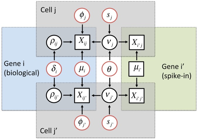
Fig 2 Graphical representation of the hierarchical model implemented in BASiCS. Diagram based on the expression counts of 2 genes (i: biological and i′: technical) at 2 cells (j and j′). Squared and circular nodes denote known observed quantities (observed expression counts and added number of spike-in mRNA molecules) and unknown elements, respectively. Whereas black circular nodes represent the random effects that play an intermediate role in our hierarchical structure, red circular nodes relate to unknown model parameters in the top layer of hierarchy in our model. Blue, green and grey areas highlight elements that are shared within a biological gene, technical gene or cell, respectively. BASiCS treats cell-specific normalising constants (ϕ j’s and s j’s) as model parameters, and estimates them by combining information across all genes. Unexplained technical noise is quantified via a single hyper-parameter θ, borrowing information across all genes and cells. Finally, BASiCS quantifies biological cell-to-cell variability via gene-specific hyper-parameters δ i, borrowing information across all cells.
Fig 2 Graphical representation of the hierarchical model implemented in BASiCS. Diagram based on the expression counts of 2 genes (i: biological and i′: technical) at 2 cells (j and j′). Squared and circular nodes denote known observed quantities (observed expression counts and added number of spike-in mRNA molecules) and unknown elements, respectively. Whereas black circular nodes represent the random effects that play an intermediate role in our hierarchical structure, red circular nodes relate to unknown model parameters in the top layer of hierarchy in our model. Blue, green and grey areas highlight elements that are shared within a biological gene, technical gene or cell, respectively. BASiCS treats cell-specific normalising constants (ϕ j’s and s j’s) as model parameters, and estimates them by combining information across all genes. Unexplained technical noise is quantified via a single hyper-parameter θ, borrowing information across all genes and cells. Finally, BASiCS quantifies biological cell-to-cell variability via gene-specific hyper-parameters δ i, borrowing information across all cells.CC BY · PubMed Central
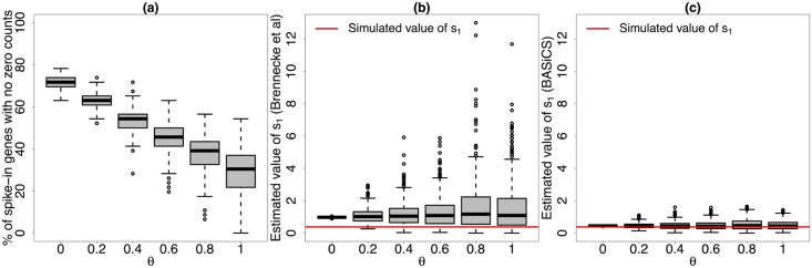
Fig 3 Simulated performance of s j’s estimates (method described in [5] and BASiCS). Based on 400 simulated datasets from the model implemented in BASiCS with the same structure as in the mouse ESC dataset (simulated parameter values defined as posterior medians of the original model fit) and 6 different values for θ. (a) percentage of the simulated spike-in genes (out of 46) without zero counts (i.e. those that can be used when calculating the estimator proposed in [5]) for different simulated values of θ. (b) and (c) estimates of s 1 (first cell) across all simulated datasets for different simulated values of θ using the method described in [5] and BASiCS (posterior medians), respectively. As the strength of unexplained technical noise increases (larger values of θ), estimates obtained using the approach described in [5] become highly unstable (we illustrated this using the first simulated cell, but the same conclusion can be obtained based on any other cell). This is due to a larger proportion of zeros among the simulated expression counts, i.e. less spike-in genes can be used when estimating s 1. In contrast, the stability of the BASiCS estimates is not substantially affected by the strength of unexplained technical noise.
Fig 3 Simulated performance of s j’s estimates (method described in [5] and BASiCS). Based on 400 simulated datasets from the model implemented in BASiCS with the same structure as in the mouse ESC dataset (simulated parameter values defined as posterior medians of the original model fit) and 6 different values for θ. (a) percentage of the simulated spike-in genes (out of 46) without zero counts (i.e. those that can be used when calculating the estimator proposed in [5]) for different simulated values of θ. (b) and (c) estimates of s 1 (first cell) across all simulated datasets for different simulated values of θ using the method described in [5] and BASiCS (posterior medians), respectively. As the strength of unexplained technical noise increases (larger values of θ), estimates obtained using the approach described in [5] become highly unstable (we illustrated this using the first simulated cell, but the same conclusion can be obtained based on any other cell). This is due to a larger proportion of zeros among the simulated expression counts, i.e. less spike-in genes can be used when estimating s 1. In contrast, the stability of the BASiCS estimates is not substantially affected by the strength of unexplained technical noise.CC BY · PubMed Central
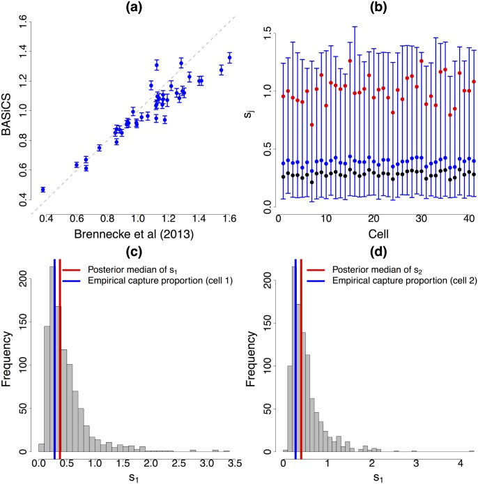
Fig 4 Normalisation. (a) and (b): for each of the 41 mouse ESCs, vertical lines represent the 95% high posterior density interval (blue dot located at the posterior median) of cell-specific normalising constants ϕ j (cellular mRNA content) and s j (interpreted in terms of capture and reverse transcription efficiency for UMI counts), respectively. While BASiCS suggests substantial heterogeneity in the total amount of molecules per cell (ϕ j), the scale of the technical counts remains stable among cells (s j). This is expected when using UMI protocols, where counts should not be affected by sequencing depth and other amplification biases. Red dots are the values estimated by the stepwise method described in [5]. There is a good agreement of the methods in terms of cellular mRNA content (ϕ j), but the estimations of s j according to [5] suggest stronger differences than what is expected when using UMI protocols. In (b), black dots represent the proportion of total spike-in molecules captured in each cell. Our estimations of the s j’s are in better agreement with these empirical measurements (suggesting BASiCS infers a more adequate reverse transcription efficiency level). (c) and (d) histogram of a Markov Chain Monte Carlo sample from s 1 and s 2, respectively. These posterior distributions are highly skewed and thence the posterior modes are a closer match to the empirical capture proportions than the corresponding posterior medians.
Fig 4 Normalisation. (a) and (b): for each of the 41 mouse ESCs, vertical lines represent the 95% high posterior density interval (blue dot located at the posterior median) of cell-specific normalising constants ϕ j (cellular mRNA content) and s j (interpreted in terms of capture and reverse transcription efficiency for UMI counts), respectively. While BASiCS suggests substantial heterogeneity in the total amount of molecules per cell (ϕ j), the scale of the technical counts remains stable among cells (s j). This is expected when using UMI protocols, where counts should not be affected by sequencing depth and other amplification biases. Red dots are the values estimated by the stepwise method described in [5]. There is a good agreement of the methods in terms of cellular mRNA content (ϕ j), but the estimations of s j according to [5] suggest stronger differences than what is expected when using UMI protocols. In (b), black dots represent the proportion of total spike-in molecules captured in each cell. Our estimations of the s j’s are in better agreement with these empirical measurements (suggesting BASiCS infers a more adequate reverse transcription efficiency level). (c) and (d) histogram of a Markov Chain Monte Carlo sample from s 1 and s 2, respectively. These posterior distributions are highly skewed and thence the posterior modes are a closer match to the empirical capture proportions than the corresponding posterior medians.CC BY · PubMed Central
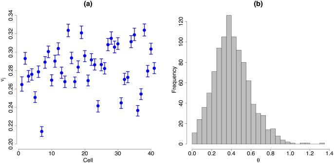
Fig 5 Cell-specific random effects linked to unexplained technical variability. (a): for each of the 41 mouse ES cells, vertical lines represent the 95% high posterior density interval (blue dot located at the posterior median) of the random effects related to unexplained technical cell-to-cell variability (ν j). (b): histogram of a Markov Chain Monte Carlo sample from θ. Posterior inference strongly suggests the presence of unexplained technical noise in gene expression measurements. In fact, the posterior distribution of θ is concentrated away from zero and—even though the posterior distributions of the s j’s are highly homogeneous across cells (see Fig 4(b))—there is a strong heterogeneity among the posterior distributions of the ν j’s (evidenced by non-overlapping 95% high posterior density intervals).
Fig 5 Cell-specific random effects linked to unexplained technical variability. (a): for each of the 41 mouse ES cells, vertical lines represent the 95% high posterior density interval (blue dot located at the posterior median) of the random effects related to unexplained technical cell-to-cell variability (ν j). (b): histogram of a Markov Chain Monte Carlo sample from θ. Posterior inference strongly suggests the presence of unexplained technical noise in gene expression measurements. In fact, the posterior distribution of θ is concentrated away from zero and—even though the posterior distributions of the s j’s are highly homogeneous across cells (see Fig 4(b))—there is a strong heterogeneity among the posterior distributions of the ν j’s (evidenced by non-overlapping 95% high posterior density intervals).CC BY · PubMed Central
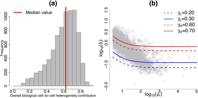
Fig 6 Biological cell-to-cell heterogeneity. (a): Histogram of the posterior medians of gene-specific biological cell-to-cell heterogeneity variance contributions σ i (defined in Eq (6)) across the 7,895 biological genes. (b): For each of the 7,895 biological genes, posterior medians of biological cell-to-cell heterogeneity term δ i (log scale) against posterior medians of expression level μ i (log scale). Red lines represent the contours in Eq (7), related to HVG (log scale) at different levels of the variance contribution threshold γ H. Blue lines represent the equivalent contours linked to LVG at different levels of the variance contribution threshold γ L. These contours were estimated based on posterior medians of ϕ j’s, s j’s and θ.
Fig 6 Biological cell-to-cell heterogeneity. (a): Histogram of the posterior medians of gene-specific biological cell-to-cell heterogeneity variance contributions σ i (defined in Eq (6)) across the 7,895 biological genes. (b): For each of the 7,895 biological genes, posterior medians of biological cell-to-cell heterogeneity term δ i (log scale) against posterior medians of expression level μ i (log scale). Red lines represent the contours in Eq (7), related to HVG (log scale) at different levels of the variance contribution threshold γ H. Blue lines represent the equivalent contours linked to LVG at different levels of the variance contribution threshold γ L. These contours were estimated based on posterior medians of ϕ j’s, s j’s and θ.CC BY · PubMed Central
Fig 7 HVG and LVG detection. (a) and (b): for each of the 7,895 biological genes, gene-specific expression rate μ i (log scale) against the probability of being HVG (πi^H(γH)) and the probability of being LVG (πi^L(γL)), respectively. Setting the EFDR and the EFNR equal to 10%, the corresponding variance contribution thresholds are γ H = 79% and γ L = 41%. Black dashed lines located at optimal (i.e. when EFDR and EFNR coincide) evidence thresholds α H = 0.7925 and α L = 0.7650, respectively. The 133 and 589 genes classified as HVG and LVG are highlighted in red and blue, respectively.
Fig 7 HVG and LVG detection. (a) and (b): for each of the 7,895 biological genes, gene-specific expression rate μ i (log scale) against the probability of being HVG (πi^H(γH)) and the probability of being LVG (πi^L(γL)), respectively. Setting the EFDR and the EFNR equal to 10%, the corresponding variance contribution thresholds are γ H = 79% and γ L = 41%. Black dashed lines located at optimal (i.e. when EFDR and EFNR coincide) evidence thresholds α H = 0.7925 and α L = 0.7650, respectively. The 133 and 589 genes classified as HVG and LVG are highlighted in red and blue, respectively.CC BY · PubMed Central
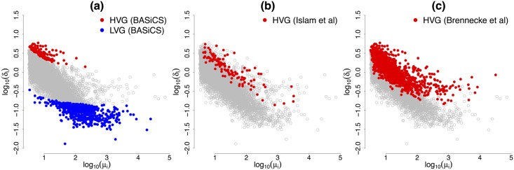
Fig 8 Comparison of HVG detection among different methods. For each of the 7,895 biological genes, posterior medians of biological cell-to-cell heterogeneity term δ i (log scale) against posterior medians of expression level μ i (log scale). While the methods described in [16] and [5] only provide a characterisation of HVG, BASiCS is able to detect those genes whose expression rates are stable among cells.
Fig 8 Comparison of HVG detection among different methods. For each of the 7,895 biological genes, posterior medians of biological cell-to-cell heterogeneity term δ i (log scale) against posterior medians of expression level μ i (log scale). While the methods described in [16] and [5] only provide a characterisation of HVG, BASiCS is able to detect those genes whose expression rates are stable among cells.CC BY · PubMed Central
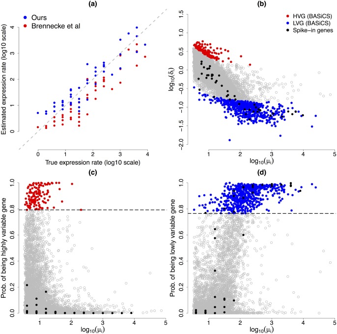
Fig 9 Cross-validation experiment. (a) true versus estimated normalised expression level μ i for each of the 46 ERCC spike-in genes (log-scale). Our estimations are gathered around the true values, except for lowly expressed technical genes, where the experiment suggests a small positive bias. Estimations according to [5] are highly correlated with the true values, however the true scale has not been recovered (not surprising as their method is not designed to estimate the right scale of the s j’s, see Fig 3). (b): Fig 8(a) superimposing (in black) estimated values for each of the 46 ERCC spike-in genes. (c) and (d): panels (c) and (d) of Fig 7 superposing (in black) estimated probabilities associated to each of the 46 ERCC spike-in genes. As expected, none of the spike-in genes were detected as HVG by our criteria. On the other hand, there is strong evidence in favour of being LVG for 21 of the technical genes (and some others are borderline according to our conservative criteria).
Fig 9 Cross-validation experiment. (a) true versus estimated normalised expression level μ i for each of the 46 ERCC spike-in genes (log-scale). Our estimations are gathered around the true values, except for lowly expressed technical genes, where the experiment suggests a small positive bias. Estimations according to [5] are highly correlated with the true values, however the true scale has not been recovered (not surprising as their method is not designed to estimate the right scale of the s j’s, see Fig 3). (b): Fig 8(a) superimposing (in black) estimated values for each of the 46 ERCC spike-in genes. (c) and (d): panels (c) and (d) of Fig 7 superposing (in black) estimated probabilities associated to each of the 46 ERCC spike-in genes. As expected, none of the spike-in genes were detected as HVG by our criteria. On the other hand, there is strong evidence in favour of being LVG for 21 of the technical genes (and some others are borderline according to our conservative criteria).CC BY · PubMed Central

Verification

Claims the paper makes

The claims and statistics of this paper haven’t been checked yet.

Run the check — free, no account needed. It reads the open-access text and checks the sources it cites.

A few free checks a day · papers already verified open instantly · results are public

Claims other papers make about this one

Each is checked against this paper’s own text: does it say what the citing paper says it does?

Self-check

Percentages, sums and reported differences re-computed from the paper’s own numbers.

The self-check needs the paper’s full text.

Citations

Cites

Show all 20 references

Cited by

Sorted by citations

Items 301–302 of 302

Metadata

Authors
Vallejos, C. A., Marioni, J. C., & Richardson, S.
Affiliations
  • European Bioinformatics Institute (GB)
  • MRC Biostatistics Unit (GB)
Corresponding author
  • Vallejos, Catalina A.
  • Marioni, John C.
  • Richardson, Sylvia
Venue
PLOS Computational Biology
Published
2015-06-24
Volume
11
Issue
6
Pages
e1004333
ISSN
  • 1553-734X (ISSN-L)
  • 1553-7358
OpenAlex
W839653734
Cited by
302
References
20
Citations by year
2026: 10 · 2025: 16 · 2024: 27 · 2023: 32 · 2022: 24 · 2021: 44 · 2020: 28 · 2019: 31 · 2018: 37 · 2017: 35 · 2016: 18
FWCI
13.02
Type
journal article
Language
en
Open access
Locations
  • PLoS Computational Biology (publishedVersion, cc-by)
  • PubMed Central (publishedVersion, cc-by)
  • PubMed (publishedVersion)
  • RePEc: Research Papers in Economics (submittedVersion)
  • DOAJ (DOAJ: Directory of Open Access Journals) (submittedVersion, cc-by-sa)
  • UCL Discovery (University College London) (submittedVersion)
  • Figshare (submittedVersion, cc-by)
  • Spiral (Imperial College London) (submittedVersion, cc-by)
Funders
  • European Bioinformatics Institute
  • Cancer Research UK (22231)
  • Medical Research Council
Topics
  • Life Sciences › Biochemistry, Genetics and Molecular Biology › Molecular Biology › Single-cell and spatial transcriptomics
  • Life Sciences › Biochemistry, Genetics and Molecular Biology › Molecular Biology › Gene expression and cancer classification
  • Life Sciences › Biochemistry, Genetics and Molecular Biology › Molecular Biology › Genomics and Phylogenetic Studies
Keywords
single-cell RNA sequencing, cellular heterogeneity, Bayesian hierarchical model, technical noise, mouse embryonic stem cells, gene expression variation
MeSH terms
Animals, Bayes Theorem, RNA, Messenger, Reproducibility of Results, Computational Biology, Oligonucleotide Array Sequence Analysis, Gene Expression Profiling, Mice, Embryonic Stem Cells, Single-Cell Analysis

About these checks

Registry, retraction, Cites and statistics results are computed, not judged, with one exception: a printed reference that no index lists is read once by a model before it counts as a citation error. Claims are extracted by a model and kept only when their quote appears verbatim in the text; each cited source is then checked, with a model’s help, for whether it says what the claim relies on. Those verdicts can be wrong — read the claim’s quote and the cited source before relying on one.

Statistics and arithmetic are recomputed, not judged.

Confidence bands are shown only for fields calibrated on our annotated test set. None is calibrated yet, so no band is shown.

What counts as a claim ›How we measure confidence ›How we check this ›

Are you an author, or do you see a problem with this page? Request a review