

The DOI matches its Crossref record; 61 of the 61 references it cites were found in a registry or an index.
Ig-VAE: Generative modeling of protein structure by direct 3D coordinate generation
Open accessPublished version of a preprint
Abstract
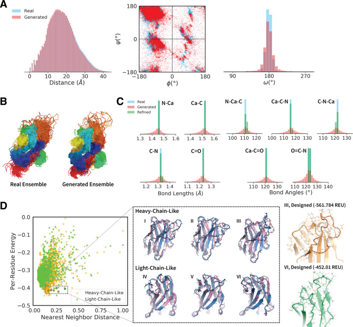
While deep learning models have seen increasing applications in protein science, few have been implemented for protein backbone generation—an important task in structure-based problems such as active site and interface design. We present a new approach to building class-specific backbones, using a variational auto-encoder to directly generate the 3D coordinates of immunoglobulins. Our model is torsion- and distance-aware, learns a high-resolution embedding of the dataset, and generates novel, high-quality structures compatible with existing design tools. We show that the Ig-VAE can be used with Rosetta to create a computational model of a SARS-CoV2-RBD binder via latent space sampling. We further demonstrate that the model’s generative prior is a powerful tool for guiding computational protein design, motivating a new paradigm under which backbone design is solved as constrained optimization problem in the latent space of a generative model.
Overview
The claims and statistics of this paper haven’t been checked yet.
Free: it reads the open-access text and checks the first 5 claims that cite a source we can check. Create a free account to check every claim.
Integrity signals
Registry
Cites
Statistics
Figures




Verification
Claims the paper makes
The claims and statistics of this paper haven’t been checked yet.
Free: it reads the open-access text and checks the first 5 claims that cite a source we can check. Create a free account to check every claim.
Claims other papers make about this one
Each is checked against this paper’s own text: does it say what the citing paper says it does?
The cited source says what the claim attributes to it.
In the citing paper
“There has been progress towards this goal and there exist approaches that address subsets of the components of this problem [53][54][55][56][63][64][65][68][69][70].”
From Computational and artificial intelligence-based methods for antibody development (2023) · cites this paper as [53]
In the citing paper
“For example, the IG-VAE model [53], which builds on previous work from the Huang group [54], generates complete backbones including all 3D coordinates by implementing a variational autoencoder trained to accurately reconstruct 3D coordinates, torsional angles, and distance maps from a learned latent space.”
From Computational and artificial intelligence-based methods for antibody development (2023) · cites this paper as [53]
Self-check
Percentages, sums and reported differences re-computed from the paper’s own numbers.
The self-check needs the paper’s full text.
Citations
Cites
(2008) · Journal of Machine Learning Research · Cited by 33,051
Auto-Encoding Variational Bayes
Kingma, D. P., & Welling, M. (2013) · arXiv · doi:10.48550/arxiv.1312.6114 · Cited by 20,067
Advances in neural information processing systems 7
(1996) · Computers & Mathematics with Applications · doi:10.1016/s0898-1221(96)90463-0 · Cited by 14,281
LIII. On lines and planes of closest fit to systems of points in space
Pearson, K. (1901) · The London, Edinburgh, and Dublin Philosophical Magazine and Journal of Science · doi:10.1080/14786440109462720 · Cited by 11,934
Improved protein structure prediction using potentials from deep learning
Senior, A. W., Evans, R., Jumper, J., Kirkpatrick, J., Sifre, L., Green, T., Qin, C., Žídek, A., Nelson, A. W. R., Bridgland, A., et al. (2020) · Nature · doi:10.1038/s41586-019-1923-7 · Cited by 3,378
PatchDock and SymmDock: servers for rigid and symmetric docking
Schneidman-Duhovny, D., Inbar, Y., Nussinov, R., & Wolfson, H. J. (2005) · Nucleic Acids Research · doi:10.1093/nar/gki481 · Cited by 3,018
Leaver-Fay (2011) · doi:10.1016/b978-0-12-381270-4.00019-6 · Cited by 1,904 · cited 2×
“All structures were idealized and relaxed under the Rosetta energy function with constraints to starting coordinates [10].”
MethodThe Rosetta All-Atom Energy Function for Macromolecular Modeling and Design
Alford, R. F., Leaver-Fay, A., Jeliazkov, J. R., O’Meara, M. J., DiMaio, F. P., Park, H., Shapovalov, M. V., Renfrew, P. D., Mulligan, V. K., Kappel, K., et al. (2017) · Journal of Chemical Theory and Computation · doi:10.1021/acs.jctc.7b00125 · Cited by 1,532
The coming of age of de novo protein design
Huang, P.-S., Boyken, S. E., & Baker, D. (2016) · Nature · doi:10.1038/nature19946 · Cited by 1,478
Self-citationImproved protein structure prediction using predicted interresidue orientations
Yang, J., Anishchenko, I., Park, H., Peng, Z., Ovchinnikov, S., & Baker, D. (2020) · Proceedings of the National Academy of Sciences · doi:10.1073/pnas.1914677117 · Cited by 1,421
Research works printed but not linked: 1
- A Riesselman, 2019, Accelerating Protein Design Using Autoregressive Generative Models., bioRxiv.
Cited by
De novo protein design by deep network hallucination
Anishchenko, I., Chidyausiku, T. M., Ovchinnikov, S., Pellock, S. J., & Baker, D. (2020) · doi:10.1101/2020.07.22.211482 · Cited by 629
Scaffolding protein functional sites using deep learning
Wang, J., Lisanza, S., Juergens, D., Tischer, D., Watson, J. L., Castro, K. M., Ragotte, R., Saragovi, A., Milles, L. F., Baek, M., et al. (2022) · Science · doi:10.1126/science.abn2100 · Cited by 487
Illuminating protein space with a programmable generative model
Ingraham, J. B., Baranov, M., Costello, Z., Barber, K. W., Wang, W., Ismail, A., Frappier, V., Lord, D. M., Ng-Thow-Hing, C., Van Vlack, E. R., et al. (2023) · Nature · doi:10.1038/s41586-023-06728-8 · Cited by 444
“22 and Supplementary Appendix L).”
Learning inverse folding from millions of predicted structures
Hsu, C., Verkuil, R., Liu, J., Lin, Z., Hie, B., Sercu, T., Lerer, A., & Rives, A. (2022) · bioRxiv (Cold Spring Harbor Laboratory) · doi:10.1101/2022.04.10.487779 · Cited by 416
Machine learning for functional protein design
Notin, P., Rollins, N., Gal, Y., Sander, C., & Marks, D. (2024) · Nature Biotechnology · doi:10.1038/s41587-024-02127-0 · Cited by 270
Metadata
- Authors
- Eguchi, R. R., Choe, C. A., & Huang, P.-S.
- Affiliations
- Stanford University (US)
- Corresponding author
- Eguchi, Raphael R.
- Choe, Christian A.
- Huang, Po-Ssu
- Venue
- PLOS Computational Biology
- Publisher
- Public Library of Science (PLoS)
- Published
- 2022-06-27
- Volume
- 18
- Issue
- 6
- Pages
- e1010271
- ISSN
- 1553-734X (ISSN-L)
- 1553-7358
- PMC
- PMC9269947
- OpenAlex
- W4283588088
- Cited by
- 141
- References
- 60
- Citations by year
- 2026: 14 · 2025: 21 · 2024: 35 · 2023: 31 · 2022: 20
- FWCI
- 8.74
- Type
- journal article
- Language
- en
- Update notices
- new_version (2022-07-08)
- Open access
- gold
- doi.org
- Licence
- Locations
- PLoS Computational Biology (publishedVersion, cc-by)
- bioRxiv (Cold Spring Harbor Laboratory) (acceptedVersion)
- PubMed Central (publishedVersion, cc-by)
- PubMed (publishedVersion)
- RePEc: Research Papers in Economics (submittedVersion)
- DOAJ (DOAJ: Directory of Open Access Journals) (submittedVersion)
- OSTI OAI (U.S. Department of Energy Office of Scientific and Technical Information) (submittedVersion)
- Funders
- School of Medicine, Stanford University
- Advanced Scientific Computing Research (SciDAC)
- Chemistry, Engineering and Medicine for Human Health, Stanford University (ChEM-H)
- National Institute of General Medical Sciences (T32GM120007.)
- Topics
- Life Sciences › Biochemistry, Genetics and Molecular Biology › Molecular Biology › Protein Structure and Dynamics
- Life Sciences › Pharmacology, Toxicology and Pharmaceutics › Drug Discovery › Computational Drug Discovery Methods
- Life Sciences › Biochemistry, Genetics and Molecular Biology › Structural Biology › Enzyme Structure and Function
- Keywords
- immunoglobulins, variational autoencoder, latent space sampling, protein design, active site design, interface design, Rosetta
- MeSH terms
- COVID-19, SARS-CoV-2, Humans, Immunoglobulins, Proteins, RNA, Viral
About these checks
Registry, retraction, Cites and statistics results are computed, not judged, with one exception: a printed reference that no index lists is read once by a model before it counts as a citation error. Claims are extracted by a model and kept only when their quote appears verbatim in the text; each cited source is then checked, with a model’s help, for whether it says what the claim relies on. Those verdicts can be wrong — read the claim’s quote and the cited source before relying on one.
Statistics and arithmetic are recomputed, not judged.
Confidence bands are shown only for fields calibrated on our annotated test set. None is calibrated yet, so no band is shown.
What counts as a claim ›How we measure confidence ›How we check this ›
Are you an author, or do you see a problem with this page? Request a review
How to cite
Cite CoChat for the checks on this page, and the paper for its own findings.
- This page
- CoChat. (2026). Citation check: Ig-VAE: Generative modeling of protein structure by direct 3D coordinate generation. https://app.cochat.ai/papers/10.1371/journal.pcbi.1010271
- The paper
- Eguchi, R. R., Choe, C. A., & Huang, P.-S. (2022). Ig-VAE: Generative modeling of protein structure by direct 3D coordinate generation. PLOS Computational Biology. https://doi.org/10.1371/journal.pcbi.1010271
Data sources
Bibliographic data: Semantic Scholar, OpenAlex, Crossref.
Contains information from the Semantic Scholar Academic Graph Datasets, made available under the ODC Attribution License (ODC-BY 1.0).
Semantic Scholar’s data is described in: Kinney, R., et al. (2023). The Semantic Scholar Open Data Platform. arXiv:2301.10140.
