

The DOI matches its Crossref record; 66 of the 67 references it cites were found in a registry or an index.
Reinforcement Learning or Active Inference?
Open accessAbstract
This paper questions the need for reinforcement learning or control theory when optimising behaviour. We show that it is fairly simple to teach an agent complicated and adaptive behaviours using a free-energy formulation of perception. In this formulation, agents adjust their internal states and sampling of the environment to minimize their free-energy. Such agents learn causal structure in the environment and sample it in an adaptive and self-supervised fashion. This results in behavioural policies that reproduce those optimised by reinforcement learning and dynamic programming. Critically, we do not need to invoke the notion of reward, value or utility. We illustrate these points by solving a benchmark problem in dynamic programming; namely the mountain-car problem, using active perception or inference under the free-energy principle. The ensuing proof-of-concept may be important because the free-energy formulation furnishes a unified account of both action and perception and may speak to a reappraisal of the role of dopamine in the brain.
Overview
The claims and statistics of this paper haven’t been checked yet.
Run the check — free, no account needed. It reads the open-access text and checks the sources it cites.
Integrity signals
Registry
Cites
Statistics
Figures
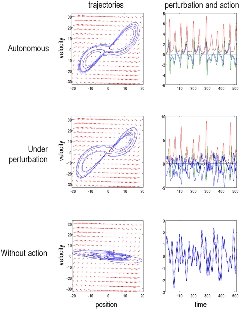
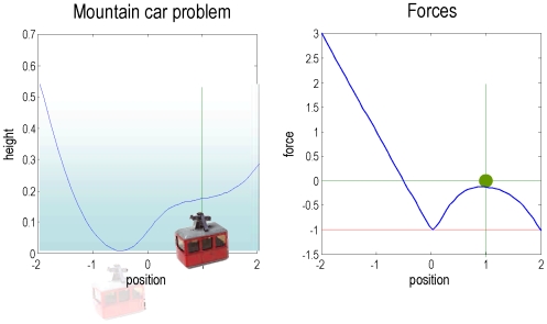
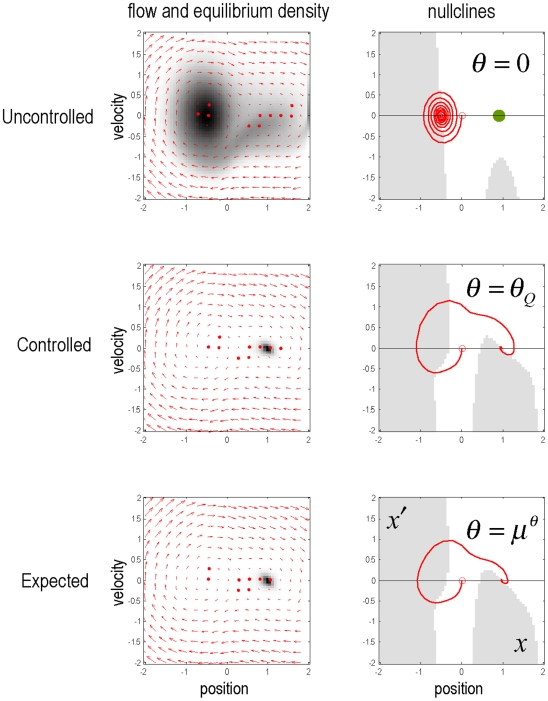
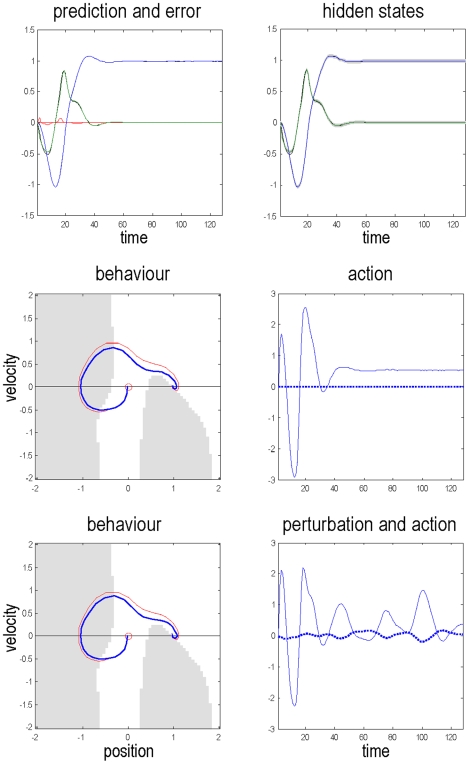
Verification
Claims the paper makes
The claims and statistics of this paper haven’t been checked yet.
Run the check — free, no account needed. It reads the open-access text and checks the sources it cites.
Claims other papers make about this one
Each is checked against this paper’s own text: does it say what the citing paper says it does?
The source backs part of the claim, not all of it — or backs it for a different population, condition or comparison.
In the citing paper
“Furthermore, this hierarchical elaboration dissolves any apparent mechanistic distinction between the optimization processes that underlie different control or learning schemes, suggesting that they are all manifestations of Active Inference – under various contexts or conditions (Friston et al., 2009).”
From Active Inference, homeostatic regulation and adaptive behavioural control (2015) · cites this paper as Friston et al., 2009
Experimental — accuracy not yet measured
Self-check
Percentages, sums and reported differences re-computed from the paper’s own numbers.
The self-check needs the paper’s full text.
Citations
Cites
A neural substrate of prediction and reward
Schultz, W., Dayan, P., & Montague, P. R. (1997) · Science · doi:10.1126/science.275.5306.1593 · Cited by 9,388
Watkins, C. J. C. H., & Dayan, P. (1992) · Machine Learning · doi:10.1007/bf00992698 · Cited by 9,083
Rescorla, R. A. (1972) · Medical Entomology and Zoology · Cited by 7,342
Autopoiesis and Cognition: The Realization of the Living
Maturana, H. R., & Varela, F. J. (1980) · Boston Studies in the Philosophy and History of Science · doi:10.1007/978-94-009-8947-4 · Cited by 5,815
Emergence of simple-cell receptive field properties by learning a sparse code for natural images
Olshausen, B. A., & Field, D. J. (1996) · Nature · doi:10.1038/381607a0 · Cited by 5,694
Rao, R. P. N., & Ballard, D. H. (1999) · Nature Neuroscience · doi:10.1038/4580 · Cited by 5,483
A theory of cortical responses.
Friston, K. (2005) · Philosophical Transactions of the Royal Society B: Biological Sciences · doi:10.1098/rstb.2005.1622 · Cited by 4,578
Self-citationPredictive reward signal of dopamine neurons
Schultz, W. (1998) · Journal of Neurophysiology · doi:10.1152/jn.1998.80.1.1 · Cited by 4,564
Classical conditioning II: Current research and theory.
Black, A. H., & Prokasy, W. F. (1972) · Appleton-Century-Crofts eBooks · Cited by 4,449
Watkins, C. J. C. H., & Dayan, P. (1992) · Machine Learning · doi:10.1023/a:1022676722315 · Cited by 3,907
Research works printed but not linked: 3
- DJC MacKay, 1995, Free-energy minimisation algorithm for decoding and cryptoanalysis., Electronics Letters, 31, 445
- T Ozaki, 1992, A bridge between nonlinear time-series models and nonlinear stochastic dynamical systems: A local linearization approach., Statistica Sin, 2, 113
- ME Tipping, 2001, Sparse Bayesian learning and the Relevance Vector Machine., J. Machine Learning Research, 1, 211
Cited by
The free-energy principle: a unified brain theory?
Friston, K. (2010) · Nature Reviews Neuroscience · doi:10.1038/nrn2787 · Cited by 8,120
Self-citationWhatever next? Predictive brains, situated agents, and the future of cognitive science
Clark, A. (2013) · Behavioral and Brain Sciences · doi:10.1017/s0140525x12000477 · Cited by 5,924
The free-energy principle: a rough guide to the brain?
Friston, K. (2009) · Trends in Cognitive Sciences · doi:10.1016/j.tics.2009.04.005 · Cited by 1,831
Self-citationAction and behavior: a free-energy formulation
Friston, K. J., Daunizeau, J., Kilner, J., & Kiebel, S. J. (2010) · Biological Cybernetics · doi:10.1007/s00422-010-0364-z · Cited by 866
“This entails adjusting the parameters to maximize the ensemble density, p(˜ x|m) at the target location, as described in Friston et al. (2009) .”
BackgroundMethodSelf-citationThe Computational Anatomy of Psychosis
Adams, R. A., Stephan, K. E., Brown, H. R., Frith, C. D., & Friston, K. J. (2013) · Frontiers in Psychiatry · doi:10.3389/fpsyt.2013.00047 · Cited by 850
“In short, active inference can be regarded www.frontiersin.org May 2013 | Volume 4 | Article 47 | 9 as equipping a generalized predictive coding scheme with classical reflex arcs: see Friston et al. (2009) and Adams et al. (2013) for details.”
BackgroundSelf-citation
Metadata
- Authors
- Friston, K. J., Daunizeau, J., & Kiebel, S. J.
- Affiliations
- Wellcome Centre for Human Neuroimaging (GB)
- Corresponding author
- Friston, Karl J.
- Venue
- PLoS ONE
- Publisher
- Public Library of Science (PLoS)
- Published
- 2009-07-29
- Volume
- 4
- Issue
- 7
- Pages
- e6421
- ISSN
- 1932-6203 (ISSN-L)
- PMC
- PMC2713351
- OpenAlex
- W2137411342
- Cited by
- 443
- References
- 67
- Citations by year
- 2026: 26 · 2025: 30 · 2024: 43 · 2023: 37 · 2022: 42 · 2021: 36 · 2020: 45 · 2019: 38 · 2018: 25 · 2017: 19 · 2016: 14 · 2015: 15 · 2014: 20 · 2013: 12 · 2012: 18
- FWCI
- 6.64
- Type
- journal article
- Language
- en
- Open access
- gold
- doi.org
- Locations
- PLoS ONE (publishedVersion, cc-by)
- Europe PMC (PubMed Central) (publishedVersion, cc-by)
- PubMed Central (publishedVersion, cc-by)
- PubMed (publishedVersion)
- Zurich Open Repository and Archive (University of Zurich) (acceptedVersion, cc-by)
- RePEc: Research Papers in Economics (submittedVersion)
- DOAJ (DOAJ: Directory of Open Access Journals) (submittedVersion, cc-by-sa)
- UCL Discovery (University College London) (submittedVersion)
- Max Planck Digital Library (submittedVersion, other-oa)
- MPG.PuRe (Max Planck Society) (submittedVersion, other-oa)
- Zurich Open Repository and Archive (University of Zurich) (submittedVersion, cc-by)
- Zurich Open Repository and Archive (University of Zurich)
- Funders
- Wellcome Trust (WT056750, 088130)
- Topics
- Life Sciences › Neuroscience › Cognitive Neuroscience › Embodied and Extended Cognition
- Physical Sciences › Computer Science › Artificial Intelligence › Reinforcement Learning in Robotics
- Social Sciences › Arts and Humanities › Philosophy › Free Will and Agency
- Keywords
- free energy principle, active inference, reinforcement learning, active perception, causal discovery, self-supervised learning, dynamic programming, mountain car problem, dopamine, perception and action
- MeSH terms
- Humans, Learning, Models, Theoretical
About these checks
Registry, retraction, Cites and statistics results are computed, not judged, with one exception: a printed reference that no index lists is read once by a model before it counts as a citation error. Claims are extracted by a model and kept only when their quote appears verbatim in the text; each cited source is then checked, with a model’s help, for whether it says what the claim relies on. Those verdicts can be wrong — read the claim’s quote and the cited source before relying on one.
Statistics and arithmetic are recomputed, not judged.
Confidence bands are shown only for fields calibrated on our annotated test set. None is calibrated yet, so no band is shown.
What counts as a claim ›How we measure confidence ›How we check this ›
Are you an author, or do you see a problem with this page? Request a review
How to cite
Cite CoChat for the checks on this page, and the paper for its own findings.
- This page
- CoChat. (2026). Citation check: Reinforcement Learning or Active Inference? https://app.cochat.ai/papers/10.1371/journal.pone.0006421
- The paper
- Friston, K. J., Daunizeau, J., & Kiebel, S. J. (2009). Reinforcement Learning or Active Inference? PLoS ONE. https://doi.org/10.1371/journal.pone.0006421
Data sources
Bibliographic data: Semantic Scholar, OpenAlex, Crossref.
Contains information from the Semantic Scholar Academic Graph Datasets, made available under the ODC Attribution License (ODC-BY 1.0).
Semantic Scholar’s data is described in: Kinney, R., et al. (2023). The Semantic Scholar Open Data Platform. arXiv:2301.10140.
