

Deep Learning with Dynamically Weighted Loss Function for Sensor-Based Prognostics and Health Management
Open accessThe DOI matches its Crossref record; 34 of the 34 references it cites were found in a registry or an index.
Abstract
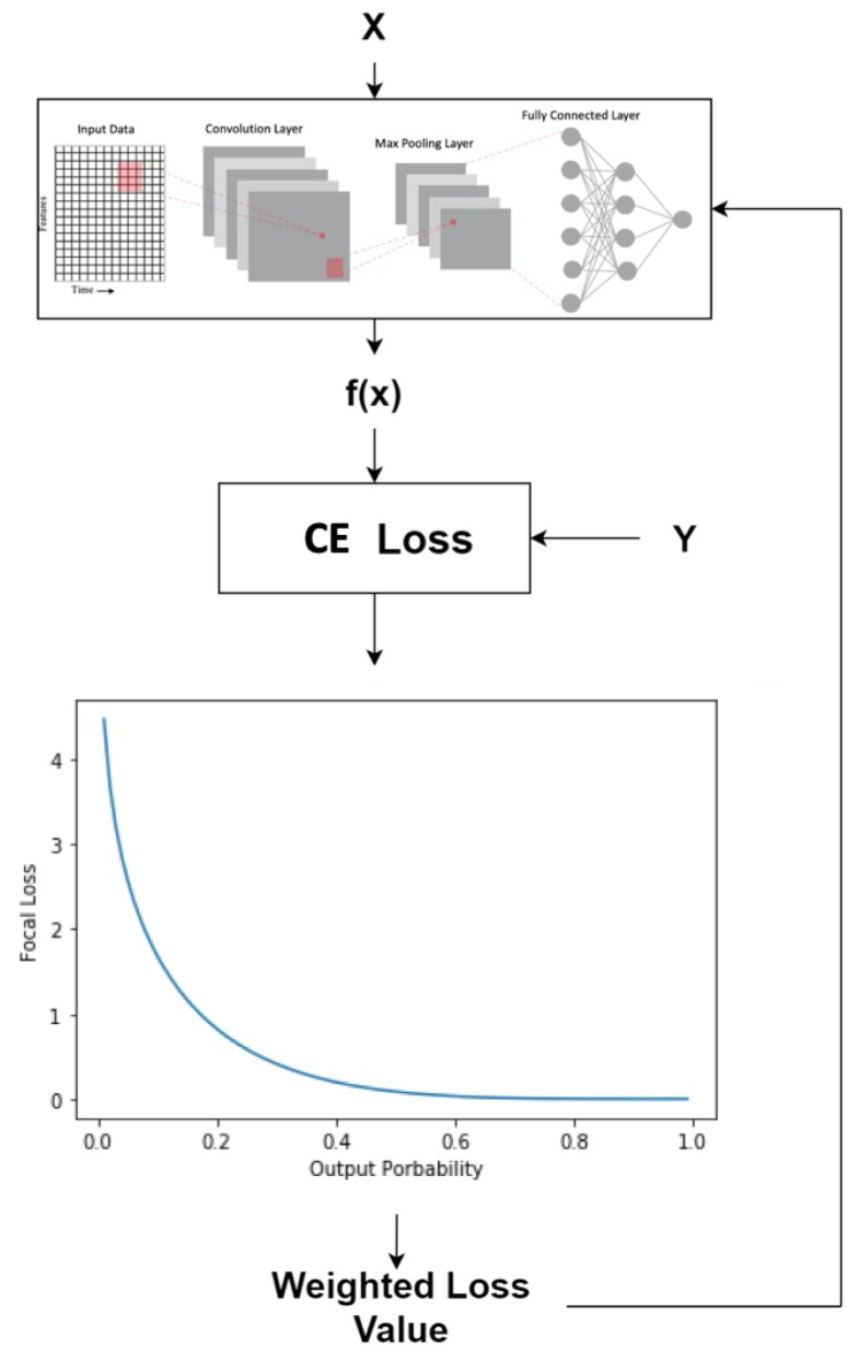
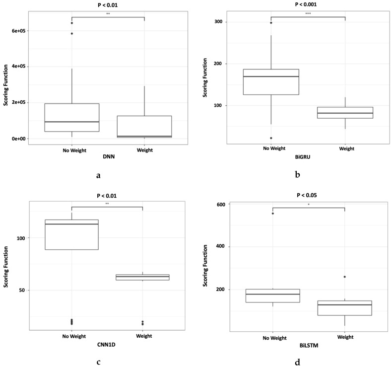
Deep learning has been employed to prognostic and health management of automotive and aerospace with promising results. Literature in this area has revealed that most contributions regarding deep learning is largely focused on the model’s architecture. However, contributions regarding improvement of different aspects in deep learning, such as custom loss function for prognostic and health management are scarce. There is therefore an opportunity to improve upon the effectiveness of deep learning for the system’s prognostics and diagnostics without modifying the models’ architecture. To address this gap, the use of two different dynamically weighted loss functions, a newly proposed weighting mechanism and a focal loss function for prognostics and diagnostics task are investigated. A dynamically weighted loss function is expected to modify the learning process by augmenting the loss function with a weight value corresponding to the learning error of each data instance. The objective is to force deep learning models to focus on those instances where larger learning errors occur in order to improve their performance. The two loss functions used are evaluated using four popular deep learning architectures, namely, deep feedforward neural network, one-dimensional convolutional neural network, bidirectional gated recurrent unit and bidirectional long short-term memory on the commercial modular aero-propulsion system simulation data from NASA and air pressure system failure data for Scania trucks. Experimental results show that dynamically-weighted loss functions helps us achieve significant improvement for remaining useful life prediction and fault detection rate over non-weighted loss function predictions.
Overview
The claims and statistics of this paper haven’t been checked yet.
Free: it reads the open-access text and checks the first 5 claims that cite a source we can check. Create a free account to check every claim.
Integrity signals
Registry
Cites
Statistics
Figures
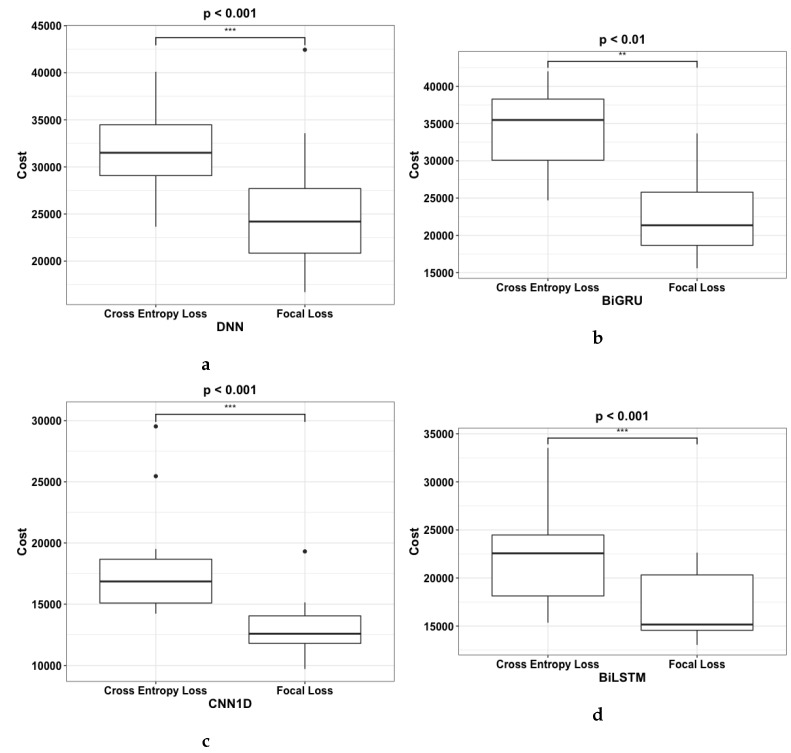
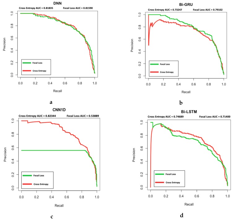
Verification
Claims the paper makes
The claims and statistics of this paper haven’t been checked yet.
Free: it reads the open-access text and checks the first 5 claims that cite a source we can check. Create a free account to check every claim.
Claims other papers make about this one
Each is checked against this paper’s own text: does it say what the citing paper says it does?
The source backs part of the claim, not all of it — or backs it for a different population, condition or comparison.
In the citing paper
“The MAE loss function maintains a constant gradient throughout the entire training process, enhancing the model's resistance to noise interference and addressing the issue of gradient explosion during training [44].”
From Prediction of Heat and Cold Loads of Factory Mushroom Houses Based on EWT Decomposition (2023) · cites this paper as [44]
Experimental — accuracy not yet measured
Self-check
Percentages, sums and reported differences re-computed from the paper’s own numbers.
The self-check needs the paper’s full text.
Citations
Cites
Hochreiter, S., & Schmidhuber, J. (1997) · Neural Computation · doi:10.1162/neco.1997.9.8.1735 · Cited by 102,318 · cited 1×
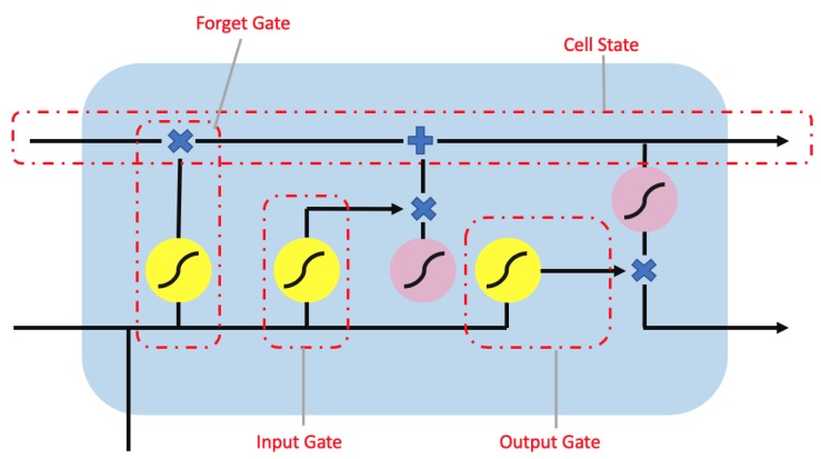
“The long short-term memory (LSTM) network [16] is a variant of the recurrent neural network [17] (RNN) designed with chain units consisting of input, forget, and output gates as shown in Figure 5.”
Background(2014) · Cited by 33,419
Focal Loss for Dense Object Detection
Lin, T.-Y., Goyal, P., Girshick, R., He, K., & Dollar, P. (2017) · 2017 IEEE International Conference on Computer Vision (ICCV) · doi:10.1109/iccv.2017.324 · Cited by 30,581
Learning Phrase Representations using RNN Encoder–Decoder for Statistical Machine Translation
Cho, K., van Merrienboer, B., Gulcehre, C., Bahdanau, D., Bougares, F., Schwenk, H., & Bengio, Y. (2014) · Proceedings of the 2014 Conference on Empirical Methods in Natural Language Processing (EMNLP) · doi:10.3115/v1/d14-1179 · Cited by 25,545 · cited 1×
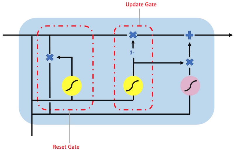
“The gated recurrent unit (GRU) [18] is proposed as alternative to LSTM.”
BackgroundA fast learning algorithm for deep belief nets
Hinton, G. E., Osindero, S., & Teh, Y.-W. (2006) · Neural Computation · doi:10.1162/neco.2006.18.7.1527 · Cited by 16,336 · cited 1×
“[20] is used to fine-tune the DBN classifier after it has been pretrained and trained.”
MethodBackpropagation Applied to Handwritten Zip Code Recognition
LeCun, Y., Boser, B., Denker, J. S., Henderson, D., Howard, R. E., Hubbard, W., & Jackel, L. D. (1989) · Neural Computation · doi:10.1162/neco.1989.1.4.541 · Cited by 11,891
Kohonen, T. (1990) · Proceedings of the IEEE · doi:10.1109/5.58325 · Cited by 8,414
Saito, T., & Rehmsmeier, M. (2015) · PLOS ONE · doi:10.1371/journal.pone.0118432 · Cited by 5,309 · cited 1×
“A PR curve is employed here as opposed to a receiver operating characteristic curve as the latter can be easily misinterpreted in highly imbalanced dataset [34].”
MethodAn overview of gradient descent optimization algorithms
Ruder, S. (2016) · arXiv · doi:10.48550/arxiv.1609.04747 · Cited by 4,962 · cited 1×
“The authors employed a conventional CNN and training was conducted using mini-batch gradient descent [29].”
MethodDamage propagation modeling for aircraft engine run-to-failure simulation
Saxena, A., Goebel, K., Simon, D., & Eklund, N. (2008) · 2008 International Conference on Prognostics and Health Management · doi:10.1109/phm.2008.4711414 · Cited by 1,954 · cited 5×
“CMAPSS is a run-to-failure gas turbine engine dataset openly sourced by NASA [12] and it is the standard dataset to compare different machine learning models for aerospace prognostics [13,14].”
BackgroundMethodInfluential
Research works printed but not linked: 1
- Figueredo G.P. Owa K. John R.I. Multi-Objective Optimization for Preventive Maintenance in Transportation: A Review Technical Report University of Nottingham Nottingham, UK 2018
Cited by
Items 101–126 of 126
Ubesigha, L., Rajapaksha, C., Mahanama, T. V., & Asanka, D. (2025) · International Conference on Advanced Research in Computing (ICARC) · doi:10.1109/icarc64760.2025.10963100 · Cited by 1
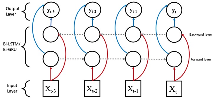
“Bi-GRU models outperform traditional methods in handling temporal dependencies for RUL predictions [16].”
Detection and Recognition of Vehicle’s Headlights Types for Surveillance Using Deep Neural Networks
Zaheer, S., Iqbal, M. J., Ahmad, I. A., Khan, S., & Khan, R. (2021) · Studies in computational intelligence · doi:10.1007/978-3-030-77939-9_20
Using In-Vehicle Monitoring Data to Assess Road Conditions of Traffic Flows
Chernyaev, I., & Evtyukov, S. A. (2022) · World of Transport and Transportation · doi:10.30932/1992-3252-2021-19-4-4
V., V. R. B., & Devi, A. J. (2022) · International Journal of Case Studies in Business IT and Education · doi:10.47992/ijcsbe.2581.6942.0177
Improving Interactive Segmentation Techniques in Medical Imaging
Pirabaharan, R. (2024) · doi:10.32920/25413817
Guasave, I. T. S. D., Delgado, G. B., Bojorquez-Delgado, J., Guasave, I. T. S. D., Obeso, A. G., & Guasave, I. T. S. D. (2024) · doi:10.61728/ae24250085
Gu, Y., Cao, J., Qian, S., Zhu, N., & Guan, W. (2024) · IEEE International Conference on Web Services (ICWS) · doi:10.1109/icws62655.2024.00111
“As a result, a sample with a higher proxy confidence is penalized more than one with lower proxy confidence for the same prediction error [49].”
BackgroundChaurasia, A. K., Greatbatch, C. J., Han, X., Gharahkhani, P., Mackey, D. A., MacGregor, S., Craig, J. E., & Hewitt, A. W. (2025) · Ophthalmology Science · doi:10.1016/j.xops.2025.100789
Forecasting Traffic Flow Under Uncertainty: A Case Study in Da Nang
Mien, D. P., Vu, T. T., & Sỹ, N. V. (2025) · Communications in computer and information science · doi:10.1007/978-981-96-4282-3_28
Large Language Model Driven Fault Diagnosis of Rotating Devices with Cross-Modal Transfer
Liu, A., Li, S., Liu, Y., & Liu, Y. (2025) · CAA Symposium on Fault Detection, Supervision and Safety for Technical Processes (SAFEPROCESS) · doi:10.1109/safeprocess67117.2025.11267953
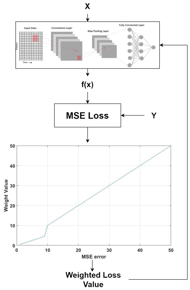
“Reference [17] explores the efficacy of deep learning for system prediction and diagnosis through the use of a weighting mechanism combined with a local loss function, employing four prevalent deep learning architectures to simulate the pneumatic system fault data of Scania trucks, demonstrating…”
Hassanzadeh, A., Krawczyk, B., Saunders, M., Wible, R., Krause, K. S., Dera, D., & van Aardt, J. (2026) · IEEE Transactions on Geoscience and Remote Sensing · doi:10.1109/tgrs.2026.3713799
“In addition, while prior studies have developed cost-sensitive weighting mechanisms to address imbalanced datasets, these approaches operate only in the univariate setting [37].”
Program Synthesis for Data Structure Conversion in the Autonomous Mobile Industry
Gál, M. (2024) · Aaltodoc (Aalto University)
Using QR Codes for Payment Card Fraud Detection
Chelouah, R., & Nwaekwu, P. (2026) · Information · doi:10.3390/info17010039
Imputation of daily rainfall in Benin using LSTM recurrent neural networks
Obada, E., Pierre, J. Z., Expédit, D., Yarou, H., Hounnondaho, F. Z., Biao, E. I., & Adechina, E. A. (2026) · International Journal of Water Resources and Environmental Engineering · doi:10.5897/ijwree2025.1131
Hasan, S. M., Raj, M. G. S., & Mitra, K. (2026) · Electronics · doi:10.3390/electronics15051108
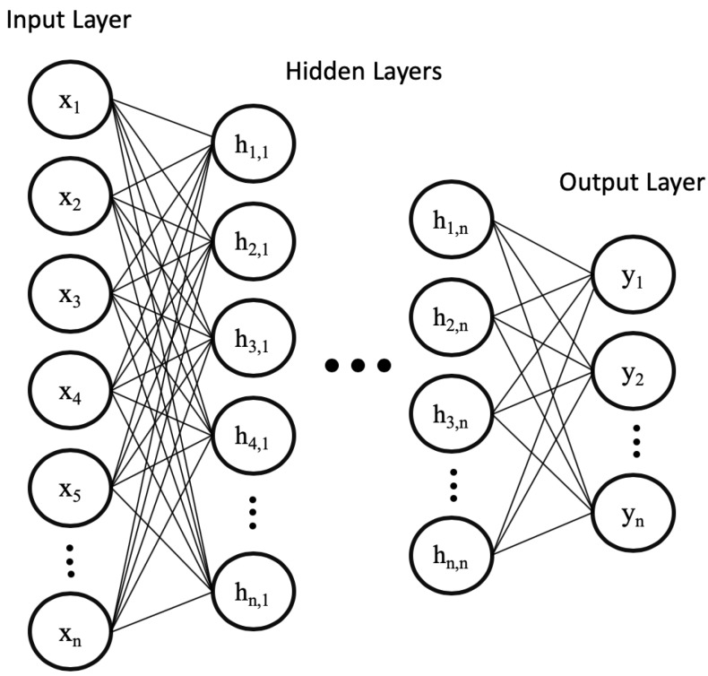
“Figure 2 represents the DFNN model [45].”
Data-efficient stress–strain prediction using optimized explainable LSTM network
Seo, H.-J., Lee, J. A., Choi, J., Seo, M. H., Oh, K.-S., & Kim, H. S. (2026) · Journal of Materials Research and Technology · doi:10.1016/j.jmrt.2026.04.075
Morphogenetic Field Loss for Unified Medical Image Segmentation
Dasgupta, S., Dey, S., Ghose, A., Mukherjee, A., & Pal, A. (2026) · IEEE International Symposium on Biomedical Imaging (ISBI) · doi:10.1109/isbi61048.2026.11515683
“Meta-learned objectives such as L2T-DLF and L2T-DLN [8, 9] adapt supervision over time, while reweighting and uncertainty-based methods [10, 11, 12] modulate pixel importance.”
Abikoye, O. C., Temitayo, E. D., Olaleru, G. I., & Abolade, J. O. (2026) · SSRN Electronic Journal · doi:10.2139/ssrn.6837692
Lin, H.-M., & Lyu, J. (2026) · Journal of Medical and Biological Engineering · doi:10.1007/s40846-026-01042-w
“This static approach cannot adapt to changing data patterns; for instance, it cannot dynamically leverage the stability of a linear model or the ability of a tree model to capture sharp fluctuations, leading to suboptimal PIs [39].”
Hong, J., & Im, T. (2026) · IEEE Access · doi:10.1109/access.2026.3707203
“Near-term predictions are inherently accurate due to their temporal proximity to the input window, whereas far-horizon predictions suffer from accumulated uncertainty; the increasing weights thus direct the optimization effort toward the more challenging temporal segment [52].”
Mraihi, A., Dimidov, V., Doorshi, R., & Khoshkangini, R. (2026) · PHM Society European Conference · doi:10.36001/phme.2026.v9i1.4963
Agarwal, S., Prabha, C., Gulhane, M., Kumar, M., & Alkhayyat, A. (2026) · Lecture notes in networks and systems · doi:10.1007/978-3-032-21901-5_21
Lei, Y., & Karimi, H. R. (2026) · Elsevier eBooks · doi:10.1016/b978-0-44-336759-5.00016-0
A Modified Genetic Algorithm-Based Deep Learning Approach for Rainfall Category Prediction
PATEL, V. B., & Morena, R. D. (2026) · Journal of Agrometeorology · doi:10.54386/jam.v28i3.3219
Metadata
- Authors
- Rengasamy, D., Jafari, M., Rothwell, B., Chen, X., & Figueredo, G. P.
- Affiliations
- University of Nottingham (GB)
- Corresponding author
- Rengasamy, Divish
- Venue
- Sensors
- Publisher
- MDPI AG
- Published
- 2020-01-28
- Volume
- 20
- Issue
- 3
- Pages
- 723
- ISSN
- 1424-8220 (ISSN-L)
- PMC
- PMC7038523
- OpenAlex
- W3003362255
- Cited by
- 118
- References
- 34
- Citations by year
- 2026: 9 · 2025: 17 · 2024: 24 · 2023: 19 · 2022: 26 · 2021: 18 · 2020: 5
- FWCI
- 8.40
- Type
- journal article
- Language
- en
- Open access
- gold
- dx.doi.org
- Licence
- Locations
- Sensors (publishedVersion, cc-by)
- PubMed Central (publishedVersion, cc-by)
- PubMed (publishedVersion)
- Repository@Nottingham (University of Nottingham) (publishedVersion, cc-by)
- Repository@Nottingham (University of Nottingham) (submittedVersion, cc-by)
- DOAJ (DOAJ: Directory of Open Access Journals) (submittedVersion, cc-by-sa)
- Funders
- H2020 Marie Skłodowska-Curie Actions (665468)
- Topics
- Physical Sciences › Engineering › Control and Systems Engineering › Machine Fault Diagnosis Techniques
- Physical Sciences › Engineering › Control and Systems Engineering › Fault Detection and Control Systems
- Physical Sciences › Engineering › Safety, Risk, Reliability and Quality › Reliability and Maintenance Optimization
- Keywords
- prognostics and health management, focal loss, remaining useful life prediction, fault detection, sensor-based condition monitoring, Scania trucks, bidirectional LSTM, bidirectional GRU, convolutional neural networks, deep feedforward neural network
- MeSH terms
- Population Health Management, Deep Learning, Algorithms, Humans, Prognosis, Biosensing Techniques, Weight Loss, Neural Networks, Computer
About these checks
Registry, retraction, Cites and statistics results are computed, not judged, with one exception: a printed reference that no index lists is read once by a model before it counts as a citation error. Claims are extracted by a model and kept only when their quote appears verbatim in the text; each cited source is then checked, with a model’s help, for whether it says what the claim relies on. Those verdicts can be wrong — read the claim’s quote and the cited source before relying on one.
Statistics and arithmetic are recomputed, not judged.
Confidence bands are shown only for fields calibrated on our annotated test set. None is calibrated yet, so no band is shown.
What counts as a claim ›How we measure confidence ›How we check this ›
Are you an author, or do you see a problem with this page? Request a review
Data sources
Bibliographic data: Semantic Scholar, OpenAlex, Crossref.
Contains information from the Semantic Scholar Academic Graph Datasets, made available under the ODC Attribution License (ODC-BY 1.0).
Semantic Scholar’s data is described in: Kinney, R., et al. (2023). The Semantic Scholar Open Data Platform. arXiv:2301.10140.
