

The DOI matches its DataCite record; 118 of the 120 references it cites were found in a registry or an index, and 2 are not checked yet.
Replica wormholes and the black hole interior
Open accessAbstract
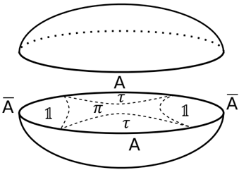
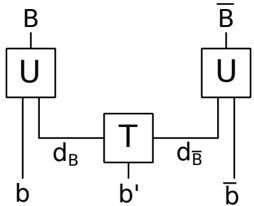
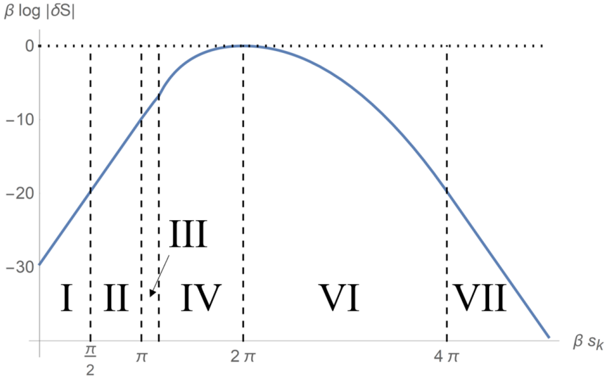
Recent work has shown how to obtain the Page curve of an evaporating black hole from holographic computations of entanglement entropy. We show how these computations can be justified using the replica trick, from geometries with a spacetime wormhole connecting the different replicas. In a simple model, we study the Page transition in detail by summing replica geometries with different topologies. We compute related quantities in less detail in more complicated models, including JT gravity coupled to conformal matter and the SYK model. Separately, we give a direct gravitational argument for entanglement wedge reconstruction using an explicit formula known as the Petz map; again, a spacetime wormhole plays an important role. We discuss an interpretation of the wormhole geometries as part of some ensemble average implicit in the gravity description.
Overview
The claims and statistics of this paper haven’t been checked yet.
Run the check — free, no account needed. It reads the open-access text and checks the sources it cites.
Integrity signals
Registry
Cites
Statistics
Figures




Verification
Claims the paper makes
The claims and statistics of this paper haven’t been checked yet.
Run the check — free, no account needed. It reads the open-access text and checks the sources it cites.
Claims other papers make about this one
Each is checked against this paper’s own text: does it say what the citing paper says it does?
The source backs part of the claim, not all of it — or backs it for a different population, condition or comparison.
In the citing paper
“It also shows in this model that results analogous to the Rényi entropy computations of [48,49] will hold not just for typical members of the ensemble defined by the Hartle-Hawking no-boundary state, but in fact for all allowed α-states.”
From Transcending the ensemble: baby universes, spacetime wormholes, and the order and disorder of black hole information (2020) · cites this paper as [49]
Experimental — accuracy not yet measuredThe source backs part of the claim, not all of it — or backs it for a different population, condition or comparison.
In the citing paper
“We then explored this construction in detail in simple topological models inspired by Jackiw-Teitelboim gravity with and without end-of-the-world branes (EOW branes, see e.g.[49,104]), and perhaps also with an extra boundary degree of freedom.Without EOW branes, there is a single asymptotically AdS boundary condition Z, for which the associated operator Z is naturally interpreted as the dimension”
From Transcending the ensemble: baby universes, spacetime wormholes, and the order and disorder of black hole information (2020) · cites this paper as [49]
Experimental — accuracy not yet measuredThe source backs part of the claim, not all of it — or backs it for a different population, condition or comparison.
In the citing paper
“Indeed, in order to explain the Rényi computations of [49] for typical members of the Hartle-Hawking ensemble some version of this compression must occur whenever the number of a priori independent states inside a quantum extremal surface exceeds the generalized entropy defined by the region outside.”
From Transcending the ensemble: baby universes, spacetime wormholes, and the order and disorder of black hole information (2020) · cites this paper as [49]
Experimental — accuracy not yet measuredThe source backs part of the claim, not all of it — or backs it for a different population, condition or comparison.
In the citing paper
“The minimum of the two dominates the path integral and gives the unitary Page curve, see [70,71] (see also [24,84]).”
From The entropy of Hawking radiation (2021) · cites this paper as [70]
Experimental — accuracy not yet measuredThe source backs part of the claim, not all of it — or backs it for a different population, condition or comparison.
In the citing paper
“More recently, it has been shown that a Petz-like map can be used to demonstrate bulk reconstruction in random tensor network toy models [52,185] of holography.”
From Holographic spacetime, black holes and quantum error correcting codes: a review (2022) · cites this paper as [52]
Experimental — accuracy not yet measured
The source backs part of the claim, not all of it — or backs it for a different population, condition or comparison.
In the citing paper
“In this Euclidean model, we represent the state of the B ∪ R system in the maximally entangled form”
From Holographic spacetime, black holes and quantum error correcting codes: a review (2022) · cites this paper as [52]
Experimental — accuracy not yet measuredThe cited source says what the claim attributes to it.
In the citing paper
“A starting point for such further investigation is the observation of [49] that the above replica trick results appear to be inconsistent with one might normally call a single welldefined theory.”
From Transcending the ensemble: baby universes, spacetime wormholes, and the order and disorder of black hole information (2020) · cites this paper as [49]
The cited source says what the claim attributes to it.
In the citing paper
“In particular, rather than taking single well-defined values, partitionfunction-like quantities seem to have both a mean value and a non-zero variance.”
From Transcending the ensemble: baby universes, spacetime wormholes, and the order and disorder of black hole information (2020) · cites this paper as [49]
The cited source says what the claim attributes to it.
In the citing paper
“Critically, [48,49] then pointed out that -at least in some contexts -this seeminglyhybrid recipe in fact follows from replica trick calculations of S rad using the gravitational path integral (and in particular that this was implicit in earlier derivations of the quantum corrected Ryu-Takayanagi [50,51] and Hubeny-Rangamani-Takayanagi [52] entropy formulae [53,54]).”
From Transcending the ensemble: baby universes, spacetime wormholes, and the order and disorder of black hole information (2020) · cites this paper as [49]
The cited source says what the claim attributes to it.
In the citing paper
“As in [49], as and discussed further in section 4, this is a version of the semiclassical Page curve [1].”
From Transcending the ensemble: baby universes, spacetime wormholes, and the order and disorder of black hole information (2020) · cites this paper as [49]
The cited source says what the claim attributes to it.
In the citing paper
“But the result is deeply related to recent successes [42,43,48,49] in reproducing various forms of the Page curve associated with the black hole information problem.”
From Transcending the ensemble: baby universes, spacetime wormholes, and the order and disorder of black hole information (2020) · cites this paper as [49]
The cited source says what the claim attributes to it.
In the citing paper
“It was then derived without holography from the gravitational path integral in [13,14], using the gravitational replica method developed earlier in [5,30].”
From Replica wormholes for an evaporating 2D black hole (2021) · cites this paper as [14]
The cited source says what the claim attributes to it.
In the citing paper
“This argument is equivalent to the derivation of the entropy in [13,14] from the defect action, but easier in practice.”
From Replica wormholes for an evaporating 2D black hole (2021) · cites this paper as [14]
The cited source says what the claim attributes to it.
In the citing paper
“This has been derived by including replica wormholes in the gravitational path integral”
From Replica wormholes for an evaporating 2D black hole (2021) · cites this paper as [14]
The cited source says what the claim attributes to it.
In the citing paper
“The island formula [1,2,9,14,29] states that the true von Neumann entropy of region R is given not by Hawking's calculation, but by an extremum of the generalized entropy,”
From Replica wormholes for an evaporating 2D black hole (2021) · cites this paper as [14]
The cited source says what the claim attributes to it.
In the citing paper
“This can be calculated directly from the action of the defect, and the result [13,14] is the island formula (2.47).”
From Replica wormholes for an evaporating 2D black hole (2021) · cites this paper as [14]
The cited source says what the claim attributes to it.
In the citing paper
“For n ∼ 1, the dynamical twist fields obey an equation of motion that extremizes the generalized entropy.Thus the twist fields become the endpoints of the island.A general argument for this based on the effective action for twist defects appears in [5,13,14,51], but in the island context, only the eternal black hole has been treated in detail [13,14].”
From Replica wormholes for an evaporating 2D black hole (2021) · cites this paper as [14]
The cited source says what the claim attributes to it.
In the citing paper
“To derive the island rule, we also need to show that the entropy derived from the replica method is equal to the generalized entropy associated to the QES.This was demonstrated from the effective action for twist defects in [13,14].”
From Replica wormholes for an evaporating 2D black hole (2021) · cites this paper as [14]
The cited source says what the claim attributes to it.
In the citing paper
“The second crucial difference is that higher topologies can contribute to the gravitational path integral.The topologies responsible for the island rule are Z n -symmetric replica wormholes [13,14].”
From Replica wormholes for an evaporating 2D black hole (2021) · cites this paper as [14]
The cited source says what the claim attributes to it.
In the citing paper
“there are other cases where non-replica-symmetric contributions to the path integral are important [14,38,64,65].”
From Replica wormholes for an evaporating 2D black hole (2021) · cites this paper as [14]
The cited source says what the claim attributes to it.
In the citing paper
“We focus on the island formula (8.2) for the entropy of the Hawking radiation [70,71].”
From The entropy of Hawking radiation (2021) · cites this paper as [70]
The cited source says what the claim attributes to it.
In the citing paper
“The idea is that very complex computations in the radiation can create wormholes that reach into that interior and pull out the information stored there [70], see also [85,86].”
From The entropy of Hawking radiation (2021) · cites this paper as [70]
The cited source says what the claim attributes to it.
In the citing paper
“Although the replica wormhole saddles produce results which are compatible with unitarity, there are crucial subtleties which are explicitly brought out by the Euclidean (Penington, Shenker, Stanford and Yang) PSSY toy model [52]”
From Holographic spacetime, black holes and quantum error correcting codes: a review (2022) · cites this paper as [52]
The cited source says what the claim attributes to it.
In the citing paper
“After this paper first appeared on arXiv, these replica trick calculations were done explicitly in [50, 51], where it was shown that the relevant topologies for the second half of the Page curve involve spacetime wormholes connecting different replicas.”
From Entanglement wedge reconstruction and the information paradox (2020) · cites this paper as [50]
The cited source says what the claim attributes to it.
In the citing paper
“The QRT prescription can be motivated via a replica trick involving Euclidean wormholes, as explored in [16-20].”
From Page curve for an evaporating black hole (2020) · cites this paper as [17]
The cited source says what the claim attributes to it.
In the citing paper
“There is a more generic derivation of the island rule (5.1) based on Euclidean replica trick techniques. This approach was investigated by two groups Almheiri et al. (2020); Penington et al. (2019).”
From Solvable models of quantum black holes: a review on Jackiw–Teitelboim gravity (2023) · cites this paper as Penington et al. (2019)
The cited source says what the claim attributes to it.
In the citing paper
“The above island formula resolves the issue with the entropy of Hawking radiation: when the semiclassical radiation entropy grows larger than the Bekenstein–Hawking entropy , the entropy is computed by choosing X to be a surface slightly in the interior of the black hole.”
From Solvable models of quantum black holes: a review on Jackiw–Teitelboim gravity (2023) · cites this paper as Penington et al. 2019
The cited source says what the claim attributes to it.
In the citing paper
“The result of this discussion is the following proposal for a formula that computes the radiation entanglement entropy in a gravitating system (Penington 2020; Almheiri et al. 2019; Penington et al. 2019; Almheiri et al. 2020):5.1”
From Solvable models of quantum black holes: a review on Jackiw–Teitelboim gravity (2023) · cites this paper as Penington et al. 2019
The cited source says what the claim attributes to it.
In the citing paper
“There have been several distinct indications (Harlow and Jafferis 2018; Penington et al. 2019; Almheiri et al. 2020; Giddings and Turiaci 2020; Stanford 2020; Engelhardt et al. 2021; Johnson 2021; Saad et al. 2021a) that the gravitational path integral is not equivalent to an ordinary quantum mechanical system (where we interpret the boundary circles as representing Euclidean time).”
From Solvable models of quantum black holes: a review on Jackiw–Teitelboim gravity (2023) · cites this paper as Penington et al. 2019
The check wasn’t confident either way, so it gives no verdict — never disputed.
In the citing paper
“With hindsight one can say that it was implicit in all of these works, and in fact moderately explicit in [49].”
From Transcending the ensemble: baby universes, spacetime wormholes, and the order and disorder of black hole information (2020) · cites this paper as [49]
Experimental — accuracy not yet measured
Self-check
Percentages, sums and reported differences re-computed from the paper’s own numbers.
The self-check needs the paper’s full text.
Citations
Cites
Particle creation by black holes
Hawking, S. W. (1975) · Communications In Mathematical Physics · doi:10.1007/bf02345020 · Cited by 13,106
Ryu, S., & Takayanagi, T. (2006) · Physical Review Letters · doi:10.1103/physrevlett.96.181602 · Cited by 4,302
Cosmological event horizons, thermodynamics, and particle creation
Gibbons, G. W., & Hawking, S. W. (1977) · Physical Review D · doi:10.1103/physrevd.15.2738 · Cited by 3,192
Hartle, J. B., & Hawking, S. W. (1983) · Physical Review D · doi:10.1103/physrevd.28.2960 · Cited by 3,027
Non-gaussian features of primordial fluctuations in single field inflationary models
Maldacena, J. (2003) · Journal of High Energy Physics · doi:10.1088/1126-6708/2003/05/013 · Cited by 2,906
Gapless spin-fluid ground state in a random quantum Heisenberg magnet
Sachdev, S., & Ye, J. (1993) · Physical Review Letters · doi:10.1103/physrevlett.70.3339 · Cited by 1,910
A covariant holographic entanglement entropy proposal
Hubeny, V. E., Rangamani, M., & Takayanagi, T. (2007) · Journal of High Energy Physics · doi:10.1088/1126-6708/2007/07/062 · Cited by 1,822 · cited 1×
“This resonates with the longstanding suspicion that some small corrections to the Hawking calculation (of order e−SBH) could be responsible for making black (1)For example [4, 5, 6, 7, 8, 9]; for a review see [10].”
BackgroundEntanglement entropy and conformal field theory
Calabrese, P., & Cardy, J. (2009) · Journal of Physics A: Mathematical and Theoretical · doi:10.1088/1751-8113/42/50/504005 · Cited by 1,688 · cited 1×
“[68])”
Average entropy of a subsystem
Page, D. N. (1993) · Physical Review Letters · doi:10.1103/physrevlett.71.1291 · Cited by 1,578
Eternal black holes in anti-de Sitter
Maldacena, J. (2003) · Journal of High Energy Physics · doi:10.1088/1126-6708/2003/04/021 · Cited by 1,555
Research works printed but not linked: 1
- C. Akers, T. Faulkner, S. Lin and P. Rath, Reflected entropy in random tensor networks, arXiv:2112.09122 [INSPIRE]. · arXiv
Cited by
Sorted by citations
Items 601–700 of 812
Ferrari, F. D. (2025) · Physical review. D/Physical review. D. · doi:10.1103/physrevd.111.l061901 · Cited by 2
Universal structure of islands in evaporating black holes
Matsuo, Y. (2025) · Journal of High Energy Physics · doi:10.1007/jhep03(2025)068 · Cited by 5
Black Hole Waterfall: a unitary phenomenological model for black hole evaporation with Page curve
Alsing, P. M. (2025) · Classical and Quantum Gravity · doi:10.1088/1361-6382/adc2eb · Cited by 3
Exponential wormhole, its quasinormal modes, and study in logarithmic f(R) gravity
Nath, P. P., & Sarma, D. (2025) · Annals of Physics · doi:10.1016/j.aop.2025.170067 · Cited by 2
On the ubiquity of (almost) contact structures in hot MQCD at intermediate coupling
Misra, A., & Yadav, G. (2025) · International Journal of Geometric Methods in Modern Physics · doi:10.1142/s0219887825502846 · Cited by 2
Generalized entropy of gravitational fluctuations
Colin-Ellerin, S., Lin, G., & Penington, G. (2025) · Journal of High Energy Physics · doi:10.1007/jhep09(2025)091 · Cited by 3
Self-citationEvaporating black holes and late-stage loss of soft hair
Cheng, P. (2022) · Physical review. D/Physical review. D. · doi:10.1103/physrevd.106.l061904 · Cited by 2
Monogamy paradox in empty flat space
Chakraborty, T., Chakravarty, J., & Paul, P. (2022) · Physical review. D/Physical review. D. · doi:10.1103/physrevd.106.086002 · Cited by 2
Late time behavior of n-point spectral form factors in Airy and JT gravities
Anegawa, T., Iizuka, N., Okuyama, K., & Sakai, K. (2023) · Journal of High Energy Physics · doi:10.1007/jhep07(2023)047 · Cited by 2
Perturbative Page curve induced by external impulse
Zhang, P. (2023) · Journal of High Energy Physics · doi:10.1007/jhep09(2023)056 · Cited by 2
Asymptotics of Weil-Petersson volumes and two-dimensional quantum gravities
Griguolo, L., Papalini, J., Russo, L., & Domenico Seminara, C. (2024) · SciPost Physics · doi:10.21468/scipostphys.17.6.156 · Cited by 2
Island formula from Wald-like entropy with backreaction
Hirano, S. (2024) · Journal of High Energy Physics · doi:10.1007/jhep02(2024)125 · Cited by 2
Sample complexity of matrix product states at finite temperature
Iwaki, A., & Hotta, C. (2024) · Physical review. B./Physical review. B · doi:10.1103/physrevb.109.224410 · Cited by 2
Phase transition in von Neumann entanglement entropy from replica symmetry breakingPreprint
Jian, S.-K., & Swingle, B. G. (2021) · arXiv (Cornell University) · doi:10.48550/arxiv.2108.11973 · Cited by 2
Baby universes, ensemble averages and factorizations with mattersPreprint
Peng, C., Tian, J., & Yu, J. (2021) · arXiv (Cornell University) · doi:10.48550/arxiv.2111.14856 · Cited by 15
Wu, S. (2024) · Journal of Physics A Mathematical and Theoretical · doi:10.1088/1751-8121/ad65a6 · Cited by 1
Holography and the Page curve of an evaporating black hole
Khodahami, A. A., & Azizi, A. (2024) · International Journal of Modern Physics D · doi:10.1142/s0218271825500038 · Cited by 2
Gravitational Algebras and Applications to Nonequilibrium Physics
Cirafici, M. (2025) · Universe · doi:10.3390/universe11010024 · Cited by 1
Islands in Bianchi type I universe
Ben-Dayan, I., Hadad, M., & Srivastava, A. (2025) · Physical review. D/Physical review. D. · doi:10.1103/physrevd.111.046015 · Cited by 1
Measurement and teleportation in the cSYK/JT correspondence
Brinster, R., Stefan Förste, B., Kruse, Y., & Natu, S. (2025) · Journal of High Energy Physics · doi:10.1007/jhep04(2025)201 · Cited by 1
Peeking Inside the Black Hole Philosophical Considerations on the AMPSS Paradox and its Resolution
Cinti, E., & Sanchioni, M. (2025) · Foundations of Physics · doi:10.1007/s10701-025-00861-2 · Cited by 2
Stable wormholes in conformal gravity
Cadoni, M., Modesto, L., Pitzalis, M., & Sanna, A. P. (2025) · Journal of Cosmology and Astroparticle Physics · doi:10.1088/1475-7516/2025/06/016 · Cited by 1
Saha, A., Chowdhury, A. R., & Gangopadhyay, S. (2025) · The European Physical Journal C · doi:10.1140/epjc/s10052-025-14579-y · Cited by 1
The entropy of disorder fields in Euclidean Schwarzschild black hole
Heymans, G. O., Rodríguez-Camargo, C. D., Scorza, G., & Svaiter, N. F. (2025) · Annals of Physics · doi:10.1016/j.aop.2025.170193 · Cited by 1
Deriving the Paradox: Original Derivation of Hawking Radiation
Cadoni, M., Mignemi, S., Pitzalis, M., & Sanna, A. P. (2025) · Springer Series in Astrophysics and Cosmology · doi:10.1007/978-981-96-6170-1_1 · Cited by 1
Toward reality of Jackiw-Teitelboim gravity in a three-component fermion chain
Huang, F.-J., Chen, Q.-H., Fu, Y., Chen, Q., Zhao, Y.-F., & Guo, W. H. (2025) · Physical review. D/Physical review. D. · doi:10.1103/8j5m-7t3p · Cited by 1
Emergent factorization of the Hilbert space at large N and the black hole information paradox
Jevicki, A., Mukherjee, D., & Yoon, J. (2025) · Physical review. D/Physical review. D. · doi:10.1103/qh7k-kpbh · Cited by 1
On the reconstruction map in JT gravity
Akers, C., Lucas, A., & Vikram, A. (2025) · Journal of High Energy Physics · doi:10.1007/jhep12(2025)045 · Cited by 2
Global symmetry violation from nonisometric codes
Baek, J.-H., & Choi, K.-S. (2025) · Physical review. D/Physical review. D. · doi:10.1103/yr3k-vj6x · Cited by 1
Random disks of constant curvature: The lattice story
Ferrari, F. D. (2025) · Physical review. D/Physical review. D. · doi:10.1103/3gb4-y8r8 · Cited by 10
Tutorial on Knots and Quantum Mechanics
Melnikov, D. (2025) · Brazilian Journal of Physics · doi:10.1007/s13538-025-01945-0 · Cited by 3
Mutual Information and the Page Curve
Chowdhury, A. R., Saha, A., & Gangopadhyay, S. (2025) · Springer proceedings in physics · doi:10.1007/978-981-95-1513-4_108 · Cited by 1
Entanglement and factorization in axion-De Sitter universes
Aguilar-Gutierrez, S. E. (2026) · Journal of High Energy Physics · doi:10.1007/jhep02(2026)036 · Cited by 6
Reflected entropy and islands in a braneworld cosmology
Basu, D., Chandra, A., & Chourasiya, H. (2026) · Journal of High Energy Physics · doi:10.1007/jhep02(2026)032 · Cited by 1
Detecting black hole microstates
Balasubramanian, V., Chan, W. K. L., & Murdia, C. (2026) · Physical review. D/Physical review. D. · doi:10.1103/yqts-ybrd · Cited by 1
Islands in Kerr–Newman black holes
Yu, M., & Ge, X.-H. (2026) · The European Physical Journal C · doi:10.1140/epjc/s10052-026-15432-6 · Cited by 1
Helping observers in closed universes reach their full potential
Higginbotham, K. (2026) · Journal of High Energy Physics · doi:10.1007/jhep03(2026)183 · Cited by 5
Replica phase transition with quantum gravity corrections
Nian, J., & Zhong, Y. (2026) · Physical review. D/Physical review. D. · doi:10.1103/s5vj-rk9g · Cited by 1
Gauge invariant Hamiltonian evolution across the black hole horizon in asymptotically AdS spacetimes
Kaushal, A., Prabhakar, N. S., & Wadia, S. R. (2026) · Physical review. D/Physical review. D. · doi:10.1103/gz2s-mqk5 · Cited by 1
How to count states in gravity
Balasubramanian, V., & Yildirim, T. P. (2026) · Physical review. D/Physical review. D. · doi:10.1103/9v3t-91qh · Cited by 1
A reverse black hole information problem
Jan De Boer, A., Hollander, J., & Rolph, A. (2026) · SciPost Physics · doi:10.21468/scipostphys.21.1.020 · Cited by 1
Rignon-Bret, A., & Vilatte, M. (2026) · Physical review. D/Physical review. D. · doi:10.1103/py7c-gxvw · Cited by 1
Chatwin-Davies, A. (2021) · doi:10.22323/1.389.0003 · Cited by 1
Replicas, averaging and factorization in the IIB matrix model
Čubrović, M. (2022) · Journal of High Energy Physics · doi:10.1007/jhep09(2022)136 · Cited by 1
Quantum Entropy Thermalization
Huang, Y., & Harrow, A. W. (2025) · Communications in Mathematical Physics · doi:10.1007/s00220-025-05268-8 · Cited by 1
A nonperturbative approach to Hawking radiation and black hole quantum hair
Wang, L. W. (2023) · Classical and Quantum Gravity · doi:10.1088/1361-6382/ad00f9 · Cited by 1
Holographic screen sequestration
Chatwin-Davies, A., Leung, P., & Remmen, G. N. (2024) · Physical review. D/Physical review. D. · doi:10.1103/physrevd.109.046003 · Cited by 1
Thermodynamics of the 3-dimensional Einstein-Maxwell system
Miyashita, S. (2024) · Journal of High Energy Physics · doi:10.1007/jhep06(2024)134 · Cited by 1
Negativity and its capacity in JT gravity
Okuyama, K., & Tachibana, T. (2024) · Journal of High Energy Physics · doi:10.1007/jhep02(2024)183 · Cited by 1
Modular average and Weyl anomaly in two-dimensional Schwarzian theory
Huang, X., & Ma, C. (2024) · Nuclear Physics B · doi:10.1016/j.nuclphysb.2024.116620 · Cited by 1
Black hole information, replica wormholes and macroscopic entanglement
Xavier Calmet, A., & Hsu, S. D. H. (2024) · International Journal of Modern Physics A · doi:10.1142/s0217751x25300017 · Cited by 1
Bounded islands in a dS 2 multiverse model
Jiang, W.-H., & Yun-song Piao, A. (2025) · Physical review. D/Physical review. D. · doi:10.1103/physrevd.111.023542 · Cited by 4
Euclidean and complex geometries from real-time computations of gravitational Rényi entropies
Held, J., Liu, X., Marolf, D. M., & Wang, Z. (2025) · Journal of High Energy Physics · doi:10.1007/jhep02(2025)136 · Cited by 1
Comments on firewalls in JT gravity with matter
Cui, C.-X., & Moshe Rozali, A. (2025) · Journal of High Energy Physics · doi:10.1007/jhep03(2025)104 · Cited by 1
Smeared end-of-the-world branes
Harvey, W., Jensen, K., & Uzu, T. (2025) · Physical review. D/Physical review. D. · doi:10.1103/physrevd.111.066017 · Cited by 1
Stretched horizon, replica trick and off-shell winding condensate, and all that
Halder, I., & Jafferis, D. L. (2025) · Journal of High Energy Physics · doi:10.1007/jhep07(2025)176 · Cited by 7
Half-wormholes in a complex SYK model
Yang, Y. (2025) · Europhysics Letters (EPL) · doi:10.1209/0295-5075/adfd7d · Cited by 4
Estimating time in quantum chaotic systems and black holes
Tang, H., Vardhan, S., & Wang, J. (2025) · SciPost Physics · doi:10.21468/scipostphys.19.4.095 · Cited by 1
Non-conformal line defect (shell operator) in AdS3/CFT2: spinning and higher point correlators
Liu, Y., & Yu, B. (2025) · Journal of High Energy Physics · doi:10.1007/jhep10(2025)161 · Cited by 2
Replica Wormholes and Quantum Hair
Xavier Calmet, A., & Hsu, S. D. H. (2025) · Fortschritte der Physik · doi:10.1002/prop.70057 · Cited by 1
Analyticity of replica correlators and modular ETH
Shyani, M. (2023) · Journal of High Energy Physics · doi:10.1007/jhep03(2023)229 · Cited by 1
Jian, S.-K., & Swingle, B. G. (2022) · Journal of High Energy Physics · doi:10.1007/jhep01(2022)083 · Cited by 1
Hawking Radiation from the Boundary Scalar Field and the Information Loss Paradox
Wang, J. (2023) · Universe · doi:10.3390/universe9030154 · Cited by 1
Tensor Field Theories: Renormalization and Random GeometryPreprint
Delporte, N. (2020) · arXiv (Cornell University) · doi:10.48550/arxiv.2010.07819 · Cited by 1
Entanglement of Initial State and Pseudo Entanglement WedgePreprint
Miyaji, M. (2021) · arXiv (Cornell University) · Cited by 1
Sovereign Takeoff Engine (STE): Observable-Only Supergrowth Laws for No-Meta Autonomous IntelligencePreprint
Takahashi, K. (2026) · Zenodo (CERN European Organization for Nuclear Research) · doi:10.5281/zenodo.18828899 · Cited by 1
Black holes to white holes II: quasi-classical scenarios for white hole evolutionPreprint
Bardeen, J. (2020) · arXiv (Cornell University) · doi:10.48550/arxiv.2007.00190
Interior of the Horizon of BTZ Black HolePreprint
Nakayama, R., & Shiohara, K. (2020) · arXiv (Cornell University) · doi:10.48550/arxiv.2008.02618
A holographic measure of quantum information exchangePreprint
Singh, H. (2021) · arXiv (Cornell University)
Laddha, A., Prabhu, S. G., Raju, S., et al. (2021) · SciPost Physics · doi:10.21468/scipost.report.2470
Patra, E. A. D. I. (2021) · Türk bilgisayar ve matematik eğitimi dergisi · doi:10.17762/turcomat.v12i2.1145
Patra, I. (2021) · Türk bilgisayar ve matematik eğitimi dergisi · doi:10.17762/turcomat.v12i2.1105
Is quantum time the classical timePreprint
Bousder, M. (2021) · arXiv (Cornell University)
Aspects of Quantum Information and AdS/CFT Duality
Balushi, A. A. (2021) · UWSpace (University of Waterloo)
Report on scipost_202010_00002v2
Chowdhury, C., Papadoulaki, O., & Raju, S. (2021) · SciPost Physics · doi:10.21468/scipost.report.2767
Report on scipost_202010_00002v1
Chowdhury, C., Papadoulaki, O., & Raju, S. (2020) · SciPost Physics · doi:10.21468/scipost.report.2083
Report on scipost_202102_00009v1
Geng, H., Karch, A., Perez-Pardavila, C., et al. (2021) · SciPost Physics · doi:10.21468/scipost.report.2703
Maximally Chaotic Dynamical System of Infinite DimensionalityPreprint
Savvidy, G. K. (2021) · arXiv (Cornell University) · doi:10.48550/arxiv.2105.12968
Information Flow In Black Hole Equilibration
Hernandez, J. (2021) · UWSpace (University of Waterloo)
Holography and quantum information exchange between systems
Singh, H. (2021) · International Journal of Modern Physics A · doi:10.1142/s0217751x21502183
Time-independence of gravitational Rényi entropies and unitarity in quantum gravity
Marolf, D. M., & Wang, Z. (2021) · Journal of High Energy Physics · doi:10.1007/jhep10(2021)196
The information horizon entropy for quantum dot and a symmetrical bathPreprint
Singh, H. (2021) · arXiv (Cornell University) · doi:10.48550/arxiv.2111.13033
Mixed-state entanglement and information recovery in thermalized states and evaporating black holesPreprint
Vardhan, S., Kudler-Flam, J., Shapourian, H., & Liu, H. (2021) · arXiv (Cornell University) · doi:10.48550/arxiv.2112.00020
Perturbative quantum consistency near black-hole horizon formation
Hofmann, S., Koegler, M., & Niedermann, F. (2021) · Physical review. D/Physical review. D. · doi:10.1103/physrevd.104.125007
Mukhametzhanov, B. (2021) · SciPost Physics · doi:10.21468/scipost.report.3459
Report on scipost_202102_00009v1
Geng, H., Karch, A., Perez-Pardavila, C., et al. (2021) · SciPost Physics · doi:10.21468/scipost.report.2752
Kruthoff, J., Mahajan, R., & Murdia, C. (2021) · SciPost Physics · doi:10.21468/scipost.report.3311
Kruthoff, J., Mahajan, R., & Murdia, C. (2021) · SciPost Physics · doi:10.21468/scipost.report.3336
Report on scipost_202107_00024v1
Basak, J. K., Basu, D., Malvimat, V., et al. (2021) · SciPost Physics · doi:10.21468/scipost.report.3313
Report on scipost_202107_00024v1
Basak, J. K., Basu, D., Malvimat, V., et al. (2021) · SciPost Physics · doi:10.21468/scipost.report.3554
Mukhametzhanov, B. (2021) · SciPost Physics · doi:10.21468/scipost.report.3536
Report on scipost_202107_00042v1
Basak, J. K., Basu, D., Malvimat, V., et al. (2021) · SciPost Physics · doi:10.21468/scipost.report.3424
Report on scipost_202107_00042v1
Basak, J. K., Basu, D., Malvimat, V., et al. (2021) · SciPost Physics · doi:10.21468/scipost.report.3495
Mukhametzhanov, B. (2021) · SciPost Physics · doi:10.21468/scipost.report.3573
Zhang, P., Liu, C., & Chen, X. (2020) · SciPost Physics · doi:10.21468/scipost.report.1662
Blommaert, A., & Kruthoff, J. (2021) · SciPost Physics · doi:10.21468/scipost.report.3888
Blommaert, A., & Kruthoff, J. (2021) · SciPost Physics · doi:10.21468/scipost.report.3852
Blommaert, A., & Kruthoff, J. (2021) · SciPost Physics · doi:10.21468/scipost.report.3844
Report on scipost_202109_00031v2
Garcı́a-Garcı́a, A. M., & Godet, V. (2022) · SciPost Physics · doi:10.21468/scipost.report.4220
Report on scipost_202109_00031v1
Garcı́a-Garcı́a, A. M., & Godet, V. (2021) · SciPost Physics · doi:10.21468/scipost.report.3882
Metadata
- Authors
- Penington, G., Shenker, S. H., Stanford, D., & Yang, Z.
- Affiliations
- Stanford University (US)
- Corresponding author
- Yang, Zhenbin
- Venue
- arXiv
- Publisher
- arXiv
- Published
- 2019
- Volume
- 2022
- Issue
- 3
- ISSN
- 1029-8479 (ISSN-L)
- arXiv
- 1911.11977
- OpenAlex
- W2991561483
- Cited by
- 809
- References
- 119
- Citations by year
- 2026: 62 · 2025: 139 · 2024: 127 · 2023: 148 · 2022: 132 · 2021: 145 · 2020: 54 · 2019: 2
- FWCI
- 17.10
- Type
- journal article
- Language
- en
- Open access
- diamond
- doi.org
- Licence
- Locations
- Journal of High Energy Physics (publishedVersion, cc-by)
- arXiv (Cornell University) (submittedVersion)
- OSTI OAI (U.S. Department of Energy Office of Scientific and Technical Information) (submittedVersion, cc-by)
- DOAJ (DOAJ: Directory of Open Access Journals) (submittedVersion)
- arXiv (Cornell University)
- Funders
- National Science Foundation (1720397)
- U.S. Department of Energy (DESC0019380)
- Simons Foundation
- Air Force Office of Scientific Research (FA9550-, FA9550-16-1-0082, FA9550-16, -16-1-, FA9550-16-1)
- Topics
- Physical Sciences › Physics and Astronomy › Nuclear and High Energy Physics › Black Holes and Theoretical Physics
- Physical Sciences › Physics and Astronomy › Nuclear and High Energy Physics › Noncommutative and Quantum Gravity Theories
- Physical Sciences › Physics and Astronomy › Atomic and Molecular Physics, and Optics › Quantum many-body systems
- Keywords
- replica wormholes, black hole evaporation, entanglement entropy, replica method, entanglement wedge reconstruction, JT gravity, conformal matter, SYK model, holography, black hole interior, ensemble average
About these checks
Registry, retraction, Cites and statistics results are computed, not judged, with one exception: a printed reference that no index lists is read once by a model before it counts as a citation error. Claims are extracted by a model and kept only when their quote appears verbatim in the text; each cited source is then checked, with a model’s help, for whether it says what the claim relies on. Those verdicts can be wrong — read the claim’s quote and the cited source before relying on one.
Statistics and arithmetic are recomputed, not judged.
Confidence bands are shown only for fields calibrated on our annotated test set. None is calibrated yet, so no band is shown.
What counts as a claim ›How we measure confidence ›How we check this ›
Are you an author, or do you see a problem with this page? Request a review
