

The DOI matches its Crossref record; 3 of the 3 references it cites were found in a registry or an index.
Palaeogeographic controls on climate and proxy interpretation
Published version of a preprint
Abstract
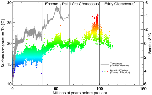
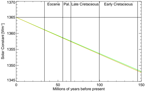
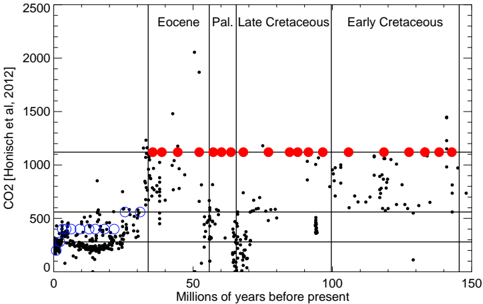
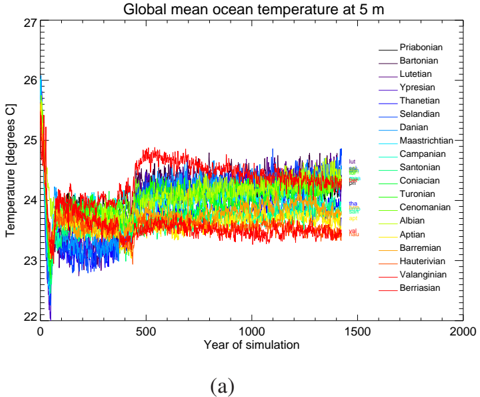
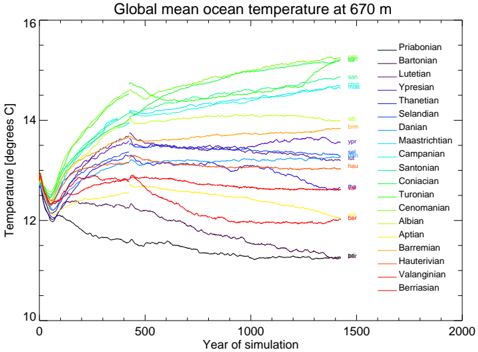
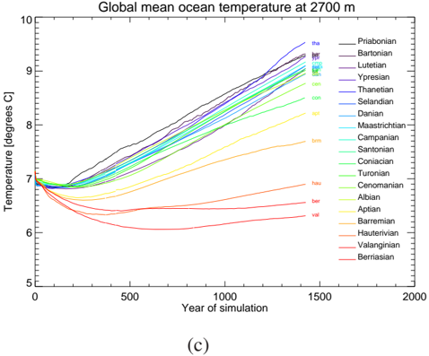
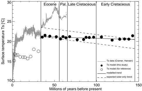
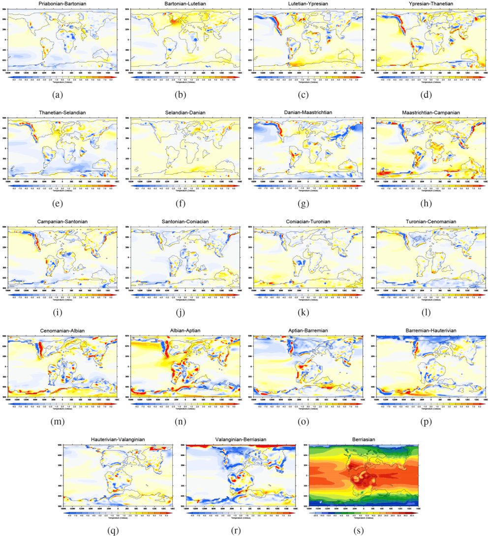
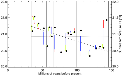
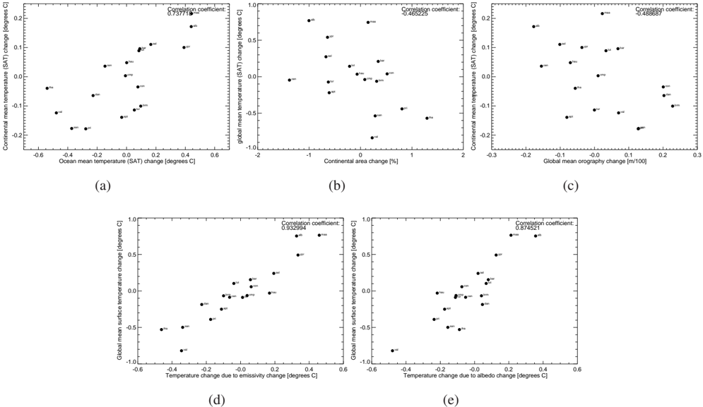
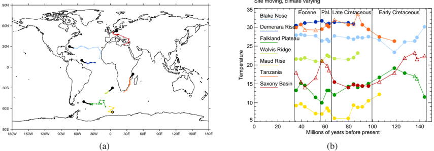
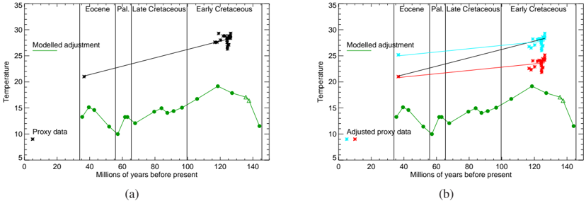
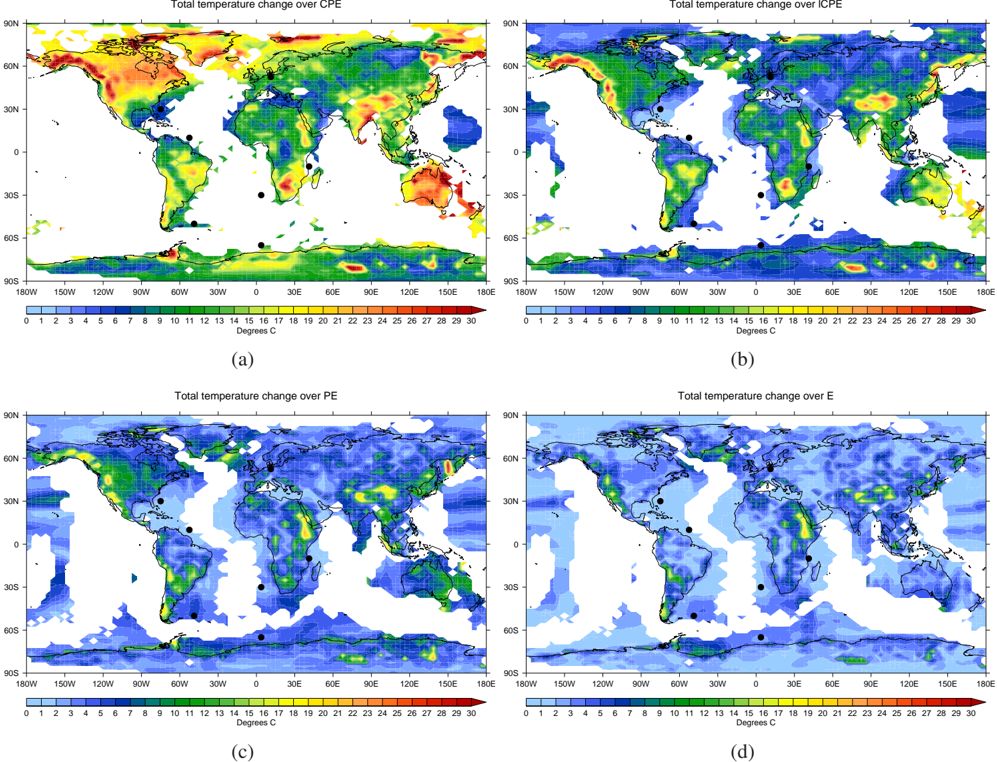
Abstract. During the period from approximately 150 to 35 million years ago, the Cretaceous–Paleocene–Eocene (CPE), the Earth was in a “greenhouse” state with little or no ice at either pole. It was also a period of considerable global change, from the warmest periods of the mid-Cretaceous, to the threshold of icehouse conditions at the end of the Eocene. However, the relative contribution of palaeogeographic change, solar change, and carbon cycle change to these climatic variations is unknown. Here, making use of recent advances in computing power, and a set of unique palaeogeographic maps, we carry out an ensemble of 19 General Circulation Model simulations covering this period, one simulation per stratigraphic stage. By maintaining atmospheric CO2 concentration constant across the simulations, we are able to identify the contribution from palaeogeographic and solar forcing to global change across the CPE, and explore the underlying mechanisms. We find that global mean surface temperature is remarkably constant across the simulations, resulting from a cancellation of opposing trends from solar and palaeogeographic change. However, there are significant modelled variations on a regional scale. The stratigraphic stage–stage transitions which exhibit greatest climatic change are associated with transitions in the mode of ocean circulation, themselves often associated with changes in ocean gateways, and amplified by feedbacks related to emissivity and planetary albedo. We also find some control on global mean temperature from continental area and global mean orography. Our results have important implications for the interpretation of single-site palaeo proxy records. In particular, our results allow the non-CO2 (i.e. palaeogeographic and solar constant) components of proxy records to be removed, leaving a more global component associated with carbon cycle change. This “adjustment factor” is used to adjust sea surface temperatures, as the deep ocean is not fully equilibrated in the model. The adjustment factor is illustrated for seven key sites in the CPE, and applied to proxy data from Falkland Plateau, and we provide data so that similar adjustments can be made to any site and for any time period within the CPE. Ultimately, this will enable isolation of the CO2-forced climate signal to be extracted from multiple proxy records from around the globe, allowing an evaluation of the regional signals and extent of polar amplification in response to CO2 changes during the CPE. Finally, regions where the adjustment factor is constant throughout the CPE could indicate places where future proxies could be targeted in order to reconstruct the purest CO2-induced temperature change, where the complicating contributions of other processes are minimised. Therefore, combined with other considerations, this work could provide useful information for supporting targets for drilling localities and outcrop studies.
Overview
The claims and statistics of this paper haven’t been checked yet.
Run the check — free, no account needed. It reads the open-access text and checks the sources it cites.
Integrity signals
Registry
Cites
Statistics
Figures
Verification
Claims the paper makes
The claims and statistics of this paper haven’t been checked yet.
Run the check — free, no account needed. It reads the open-access text and checks the sources it cites.
Claims other papers make about this one
Each is checked against this paper’s own text: does it say what the citing paper says it does?
In the citing paper
“HadCM3L has contributed to the Coupled Mode Intercomparison Project experiments demonstrating skill at reproducing the modern-day climate (71, 72) and has been used for an array of different paleoclimate experiments (73–75).”
From Asteroid impact, not volcanism, caused the end-Cretaceous dinosaur extinction (2020) · cites this paper as [73]
Self-check
Percentages, sums and reported differences re-computed from the paper’s own numbers.
The self-check needs the paper’s full text.
Citations
Cites
Solar interior structure and luminosity variations
Gough, D. O. (1981) · Solar Physics · doi:10.1007/bf00151270 · Cited by 798
Climate sensitivity, sea level and atmospheric carbon dioxide
Hansen, J., Sato, M., Russell, G., & Kharecha, P. (2013) · Philosophical Transactions of the Royal Society A: Mathematical, Physical and Engineering Sciences · doi:10.1098/rsta.2012.0294 · Cited by 660
Zhou, J., Poulsen, C. J., Pollard, D., & White, T. S. (2008) · Paleoceanography · doi:10.1029/2008pa001596 · Cited by 128
Research works printed but not linked: 65
- Barrera, E. and Huber, B. T.: Evolution of Antarctic waters during the Maestrichtian: Foraminifer oxygen and carbon isotope ratios, ODP Leg 113, in Barker, P. F., Kennett, J. P., et al., Proceedings of the Ocean Drilling Program, scientific results: College Station, Texas, Ocean Drilling Program, 113, 813–823, 1990. · DOI
- Barron, E. J. and Peterson, W. H.: Mid-Cretaceous ocean circulation: results from model sensitivity studies, Paleoceanography, 5, 319–337, 1990. · DOI
- Barron, E. J. and Washington, W. M.: The role of geographic variables in explaining paleoclimates: results from Cretaceous Climate Model sensitivity studies, J. Geophys. Res., 89, 1267–1279, 1984. · DOI
- Barron, E. J., Sloan II, J. L., and Harrison, C. G. A.: Potential significance of land-sea distribution and surface albedo variations as a climatic forcing factor; 180 M.Y. to the present, Palaeogeogr. Palaeocl., 30, 17–40, 1980. · DOI
- Barron, E. J., Fawcett, P. J., Peterson, W. H., Pollard, D., and Thompson, S. L.: A `simulation' of mid-Cretaceous climate, Paleoceanography, 10, 953–962, 1995. · DOI
- Beerling, D. and Royer, D.: Convergent Cenozoic CO2 history, Nat. Geosci., 4, 418–420, 2011. · DOI
- Beerling, D. J., Fox, A., Stevenson, D. S., and Valdes, P. J.: Enhanced chemistry-climate feedbacks in past greenhouse worlds, P. Natl. Acad. Sci. USA, 108, 9770–9775, 2011. · DOI · Paper page
- Bice, K. L. and Marotzke, J.: Could changing ocean circulation have destabilized methane hydrate at the Paleocene/Eocene boundary?, Paleoceanography, 17, 1018, https://doi.org/10.1029/2001PA000678, 2002. · DOI
- Bice, K. L., Huber, B. T., and Norris, R. D.: Extreme polar warmth during the Cretaceous greenhouse? Paradox of the late Turonian δ18O record at Deep Sea Drilling Project Site 511, Paleoceanography, 18, 1031, https://doi.org/10.1029/2002PA000848, 2003. · DOI
- Bice, K. L., Birgel, D., Meyers, P. A., Dahl, K. A., Hinrichs, K.-U., and Norris, R. D.: A multiple proxy and model study of Cretaceous upper ocean temperatures and atmospheric CO2 concentrations, Paleoceanography, 21, PA2002, https://doi.org/10.1029/2005PA001203, 2006. · DOI
- Bornemann, A., Norris, R., Friedrich, O., Beckmann, B., Schouten, S., Sinninghe-Damsté, J., Vogel, J., Hofmann, P., and Wagner, T.: Isotopic evidence for glaciation during the Cretaceous supergreenhouse, Science, 319, 189–192, 2008. · DOI
- Bradshaw, C. D., Lunt, D. J., Flecker, R., Salzmann, U., Pound, M. J., Haywood, A. M., and Eronen, J. T.: The relative roles of CO2 and palaeogeography in determining late Miocene climate: results from a terrestrial model-data comparison, Clim. Past, 8, 1257–1285, https://doi.org/10.5194/cp-8-1257-2012, 2012. · DOI
- Caballero, R. and Huber, M.: State-dependent climate sensitivity in past warm climates and its implications for future climate projections, P. Natl. Acad. Sci. USA, 110, 14162–14167, 2013. · DOI
- Caldeira, K. and Kasting, J. F.: The life span of the biosphere revisited, Nature, 360, 721–723, 1992. · DOI
- Cox, P., Betts, R., Bunton, C., Essery, R., Rowntree, P. R., and Smith, J.: The impact of new land-surface physics on the GCM simulation and climate sensitivity, Clim. Dynam., 15, 183–203, 1999. · DOI
- Cox, P. M., Betts, R. A., Jones, C. D., Spall, S. A., and Totterdell, I. J.: Modelling vegetation and the carbon cycle as interactive elements of the climate system, in: Meteorology at the Millennium, edited by: Pearce, R., Academic Press, San Diego CA, USA, 259–279, 2001. · DOI
- Cramer, B. S., Toggweiler, J. R., Wright, J. D., Katz, M. E., and Miller, K. G.: Ocean overturning since the Late Cretaceous: inferences from a new benthic foraminiferal isotope compilation, Paleoceanography, 24, PA4216, https://doi.org/10.1029/2008PA001683, 2009. · DOI
- Donnadieu, Y., Pierrehumbert, R., Jacob, R., and Fluteau, F.: Modelling the primary control of paleogeography on Cretaceous climate, Earth Planet. Sc. Lett., 248, 426–437, 2006. · DOI
- Donnadieu, Y., Goddéris, Y., and Bouttes, N.: Exploring the climatic impact of the continental vegetation on the Mezosoic atmospheric CO2 and climate history, Clim. Past, 5, 85–96, https://doi.org/10.5194/cp-5-85-2009, 2009. · DOI
- Donnadieu, Y., Pucéat, E., Moiraud, M., Guillocheau, F., and Deconinck, J.: A better-ventilated ocean triggered by Late Cretaceous changes in continental configuration, Nature Communications, 7, 10316, https://doi.org/10.1038/ncomms10316, 2016. · DOI
- Erbacher, J., Friedrich, O., Wilson, P., Lehmann, J., and Weiss, W.: Short-term warming events during the boreal Albian (mid-Cretaceous), Geology, 39, 223–226, 2011. · DOI
- Forster, A., Schouten, S., Baas, M., and Sinninghe Damste, J. S.: Mid-Cretaceous (Albian–Santonian) sea surface temperature record of the tropical Atlantic Ocean, Geology, 35, 919–922, 2007. · DOI
- Foster, G. L., Lunt, D. J., and Parrish, R. R.: Mountain uplift and the glaciation of North America – a sensitivity study, Clim. Past, 6, 707–717, https://doi.org/10.5194/cp-6-707-2010, 2010. · DOI
- Franks, P. J., Royer, D. L., Beerling, D. J., de Water, P. K. V., Cantrill, D. J., Barbour, M. M., and Berry, J. A.: New constraints on atmospheric CO2 concentration for the Phanerozoic, Geophys. Res. Lett., 41, 4685–4694, https://doi.org/10.1002/2014GL060457, 2014. · DOI
- Friedrich, O., Erbacher, J., Moriya, K., Wilson, P., and Kuhnert, H.: Warm saline intermediate waters in the Cretaceous tropical Atlantic Ocean, Nat. Geosci., 1, 453–457, 2008. · DOI
- Friedrich, O., Herrle, J. O., Wilson, P. A., Cooper, M. J., Erbacher, J., and Hemleben, C.: Early Maastrichtian carbon cycle perturbation and cooling event: Implications from the South Atlantic Ocean, Paleoceanography, 24, PA2211, https://doi.org/10.1029/2008PA001654, 2009. · DOI
- Friedrich, O., Norris, R. D., and Erbacher, J.: Evolution of middle to Late Cretaceous oceans – a 55 m.y. record of Earth's temperature and carbon cycle, Geology, 40, 107–110, 2012. · DOI
- Gordon, C., Cooper, C., Senior, C. A., Banks, H., Gregory, J. M., Johns, T. C., Mitchell, J. F. B., and Wood, R. A.: The simulation of SST, sea ice extents and ocean heat transports in a version of the Hadley Centre coupled model without flux adjustments, Clim. Dynam., 16, 147–168, 2000. · DOI
- Honisch, B., Ridgwell, A., Schmidt, D. N., Thomas, E., Gibbs, S. J., Sluijs, A., Zeebe, R., Kump, L., Martindale, R. C., Greene, S. E., Kiessling, W., Ries, J., Zachos, J. C., Royer, D. L., Barker, S., Marchitto, T. M., Moyer, R., Pelejero, C., Ziveri1, P., Foster, G. L., and Williams, B.: The geological record of ocean acidification, Science, 335, 1058–1063, 2012. · DOI
- Huber, B. T., Hodell, D. A., and Hamilton, C. P.: Middle-Late Cretaceous climate of the southern high latitudes: stable isotopic evidence for minimal equator-to- pole thermal gradients, Geol. Soc. Am. Bull., 107, 1164–1191, 1995. · DOI
- Huber, B. T., Norris, R. D., and MacLeod, K. G.: Deep-sea paleotemperature record of extreme warmth during the Cretaceous, Geology, 30, 123–126, 2002. · DOI
- Huber, M. and Caballero, R.: The early Eocene equable climate problem revisited, Clim. Past, 7, 603–633, https://doi.org/10.5194/cp-7-603-2011, 2011. · DOI
- Inglis, G. N., Farnsworth, A., Lunt, D., Foster, G., Hollis, C., Pagani, M., Jardine, P., Pearson, P., Markwick, P., Raynman, L., Galsworthy, A., and Pancost, R.: Descent towards the icehouse: Eocene sea surface cooling inferred from GDGT distributions, Paleoceanography, 30, 1000–1020, https://doi.org/10.1002/2014PA002723, 2015. · DOI
- Irvine, P. J., Gregoire, L. J., Lunt, D. J., and Valdes, P. J.: An efficient method to generate a perturbed parameter ensemble of a fully coupled AOGCM without flux-adjustment, Geosci. Model Dev., 6, 1447–1462, https://doi.org/10.5194/gmd-6-1447-2013, 2013. · DOI
- Jenkyns, H. C., Schouten-Huibers, L., Schouten, S., and Sinninghe Damsté, J. S.: Warm Middle Jurassic-Early Cretaceous high-latitude sea-surface temperatures from the Southern Ocean, Clim. Past, 8, 215–226, https://doi.org/10.5194/cp-8-215-2012, 2012. · DOI
- Kennedy, A., Farnsworth, A., Lunt, D., and Lear, C.: Palaeogeographic control on the atmospheric and oceanic impacts of Antarctic glaciation at the Eocene–Oligocene boundary, Philos. T. R. Soc. A, 373, 20140419, https://doi.org/10.1098/rsta.2014.0419, 2015. · DOI · Paper page
- Kim, J. H., Van Der Meer, J., Schouten, S., Helmke, P., Willmott, V., Sangiorgi, F., Koç, N., Hopmans, E. C., and Sinninghe Damsté, J. S.: New indices and calibrations derived from the distribution of crenarchaeal isoprenoid tetraether lipids: Implications for past sea surface temperature reconstructions, Geochim. Cosmochim. Ac., 74, 4639–4654, 2010. · DOI
- Lauderdale, J. M., Naveira Garabato, A. C., Oliver, K. I., Follows, M. J., and Williams, R. G.: Wind-driven changes in Southern Ocean residual circulation, ocean carbon reservoirs and atmospheric CO2, Clim. Dynam., 41, 2145–2164, 2013. · DOI
- Linnert, C., Robinson, S., Lees, J., Bown, P., Perez-Rodriguez, I., Petrizzo, M., Falzoni, F., Littler, K., Arz, J., and Russell, E.: Evidence for global cooling in the Late Cretaceous, Nature Communications, 5, 4194, https://doi.org/10.1038/ncomms5194, 2014. · DOI
- Littler, K., Robinson, S., Bown, P., Nederbragt, A., and Pancost, R.: High sea-surface temperatures during the Early Cretaceous Epoch, Nat. Geosci., 4, 169–172, 2011. · DOI
- Loptson, C. A., Lunt, D. J., and Francis, J. E.: Investigating vegetation-climate feedbacks during the early Eocene, Clim. Past, 10, 419–436, https://doi.org/10.5194/cp-10-419-2014, 2014. · DOI
- Lunt, D. J., Valdes, P. J., Dunkley Jones, T., Ridgwell, A., Haywood, A. M., Schmidt, D. N., Marsh, R., and Maslin, M.: CO2-driven ocean circulation changes as an amplifier of Paleocene–Eocene thermal maximum hydrate destabilization, Geology, 38, 875–878, 2010. · DOI
- Lunt, D. J., Dunkley Jones, T., Heinemann, M., Huber, M., LeGrande, A., Winguth, A., Loptson, C., Marotzke, J., Roberts, C. D., Tindall, J., Valdes, P., and Winguth, C.: A model-data comparison for a multi-model ensemble of early Eocene atmosphere-ocean simulations: EoMIP, Clim. Past, 8, 1717–1736, https://doi.org/10.5194/cp-8-1717-2012, 2012. · DOI
- Luyendyk, B. P., Forsyth, D., and Phillips, J. D.: Experimental approach to the palecirculation of the oceanic surface waters, Geol. Soc. Am. Bull., 83, 2649–2664, 1972. · DOI
- MacLeod, K., Huber, B., Berrocoso, A., and Wendler, I.: A stable and hot Turonian without glacial δ18O excursions is indicated by exquisitely preserved Tanzanian Foraminifera, Geology, 41, 1083–1086, 2013. · DOI
- Markwick, P. J. and Valdes, P. J.: Palaeo-digital elevation models for use as boundary conditions in coupled ocean–atmosphere GCM experiments: a Maastrichtian (late Cretaceous) example, Palaeogeogr. Palaeocl., 213, 37–63, 2004. · DOI
- Markwick, P. J.: The palaeogeographic and palaeoclimatic significance of climate proxies for data-model comparisons, in Deep time perspectives on climate change: marrying the signal from computer models and biological proxies, edited by: Williams, M., Haywood, A. M., Gregory, J. F., and Schmidt, D. N., The Micropalaeontological Society Special Publications, Geological Society of London, London, 251–312, 2007. · DOI
- Martinez-Boti, M., Foster, G., Chalk, T., Rohling, E., Sexton, P., Lunt, D., Pancost, R., Badger, M., and Schmidt., D.: Plio–Pleistocene climate sensitivity evaluated using high-resolution CO2 records, Nature, 518, 49–54, 2015. · DOI
- Otto-Bliesner, B. L., Brady, E. C., and Shields, C.: Late Cretaceous ocean: Coupled simulations with the National Center for Atmospheric Research Climate System Model, J. Geophys. Res., 107, 4019, https://doi.org/10.1029/2008PA001654, 2002. · DOI
- Pagani, M., Huber, M., Liu, Z., Bohaty, S. M., Henderiks, J., Sijp, W., Krishnan, S., and DeConto, R. M.: The role of carbon dioxide during the onset of Antarctic glaciation, Science, 334, 1261–1264, 2011. · DOI
- Pearson, P. N., Foster, G. L., and Wade, B. S.: Atmospheric carbon dioxide through the Eocene–Oligocene climate transition, Nature, 461, 1110–1113, 2009. · DOI
- Poulsen, C. J., Barron, E. J., Arthur, M. A., and Peterson, W. H.: Response of the mid-Cretaceous global oceanic circulation to tectonic and CO2 forcings, Paleoceanography, 16, 1–17, 2001. · DOI
- Poulsen, C. J., Gendaszek, A. S., and Jacob, R. L.: Did the rifting of the Atlantic Ocean cause the Cretaceous thermal maximum?, Geology, 31, 115–118, 2003. · DOI
- Poulsen, C. J., Pollard, D., and White, T. S.: General circulation model simulation of the δ18O content of continental precipitation in the middle Cretaceous: a model–proxy comparison, Geology, 35, 199–202, 2007. · DOI
- Raymo, M. E., Ruddiman, W. F., and Froelich, P. N.: Influence of late Cenozoic mountain building on ocean geochemical cycles, Geology, 16, 649–653, 1988. · DOI · Paper page
- Royer, D., Pagani, M., and Beerling, D. J.: Geobiological constraints on Earth system sensitivity to CO2 during the Cretaceous and Cenozoic, Geobiology, 10, 298–310, 2012. · DOI · Paper page
- Ruddiman, W. F. and Kutzbach, J. E.: Forcing of Late Cenozoic Northern Hemisphere climate by plateau uplift in southern Asia and the American West, J. Geophys. Res.-Atmos., 94, 18409–18427, 1989. · DOI
- Scotese, C.: Atlas of Earth History, University of Texas, Arlington, available at: http://www.academia.edu/9730874/Atlas_of_Earth_History, ISBN: 0-9700020-0-9, 2001.
- Sellwood, B. W., Price, G. D., and Valdes, P. J.: Cooler estimates of Cretaceous temperatures, Nature, 370, 453–455, 1994. · DOI
- Spicer, R. A., Ahlberg, A., Herman, A. B., Hofmann, C.-C., Raikevich, M., Valdes, P. J., and Markwick, P. J.: The Late Cretaceous continental interior of Siberia: a challenge for climate models, Earth Planet. Sc. Lett., 267, 228–235, 2008. · DOI
- Upchurch, G. R., Kiehl, J., Shields, C., Scherer, J., and Scotese, C.: Latitudinal temperature gradients and high-latitude temperatures during the latest Cretaceous: Congruence of geologic data and climate models, Geology, 43, 683–686, 2015. · DOI
- Winguth, A., Shellito, C., Shields, C., and Winguth, C.: Climate response at the Paleocene–Eocene thermal maximum to greenhouse gas forcing – a model study with CCSM3, J. Climate, 23, 2562–2584, 2010. · DOI
- Zhang, Y., Pagani, M., Liu, Z., Bohaty, S. M., and DeConto, R.: A 40-million-year history of atmospheric CO2, Philos. T. R. Soc. A, 371, 20130096, https://doi.org/10.1098/rsta.2013.0096, 2013. · DOI
- Zhang, Z., Nisancioglu, K. H., Flatøy, F., Bentsen, M., Bethke, I., and Wang, H.: Tropical seaways played a more important role than high latitude seaways in Cenozoic cooling, Clim. Past, 7, 801–813, https://doi.org/10.5194/cp-7-801-2011, 2011. · DOI
- Zhou, J., Poulsen, C. J., Rosenbloom, N., Shields, C., and Briegleb, B.: Vegetation-climate interactions in the warm mid-Cretaceous, Clim. Past, 8, 565–576, https://doi.org/10.5194/cp-8-565-2012, 2012. · DOI
Cited by
Asteroid impact, not volcanism, caused the end-Cretaceous dinosaur extinction
Chiarenza, A. A., Farnsworth, A., Mannion, P. D., Lunt, D. J., Valdes, P. J., Morgan, J. V., & Allison, P. A. (2020) · Proceedings of the National Academy of Sciences · doi:10.1073/pnas.2006087117 · Cited by 228
Self-citationde Winter, N. J., Müller, I. A., Kocken, I. J., Thibault, N., Ullmann, C. V., Farnsworth, A., Lunt, D. J., Claeys, P., & Ziegler, M. (2021) · Communications Earth & Environment · doi:10.1038/s43247-021-00193-9 · Cited by 52
Self-citation
Metadata
- Authors
- Lunt, D. J., Farnsworth, A., Loptson, C., Foster, G. L., Markwick, P., O'Brien, C. L., Pancost, R. D., Robinson, S. A., & Wrobel, N.
- Venue
- Climate of the Past
- Publisher
- Copernicus GmbH
- Published
- 2016-05-20
- Volume
- 12
- Issue
- 5
- Pages
- 1181-1198
- ISSN
- 1814-9332
- Cited by
- 145
- References
- 3
- Language
- en
- Funders
- Natural Environment Research Council (NE/K014757/1, NE/I005714/1, NE/I005501/2, NE/K012479/1)
About these checks
Registry, retraction, Cites and statistics results are computed, not judged, with one exception: a printed reference that no index lists is read once by a model before it counts as a citation error. Claims are extracted by a model and kept only when their quote appears verbatim in the text; each cited source is then checked, with a model’s help, for whether it says what the claim relies on. Those verdicts can be wrong — read the claim’s quote and the cited source before relying on one.
Statistics and arithmetic are recomputed, not judged.
Confidence bands are shown only for fields calibrated on our annotated test set. None is calibrated yet, so no band is shown.
What counts as a claim ›How we measure confidence ›How we check this ›
Are you an author, or do you see a problem with this page? Request a review
How to cite
Cite CoChat for the checks on this page, and the paper for its own findings.
- This page
- CoChat. (2026). Citation check: Palaeogeographic controls on climate and proxy interpretation. https://app.cochat.ai/papers/10.5194/cp-12-1181-2016
- The paper
- Lunt, D. J., Farnsworth, A., Loptson, C., Foster, G. L., Markwick, P., O'Brien, C. L., Pancost, R. D., Robinson, S. A., & Wrobel, N. (2016). Palaeogeographic controls on climate and proxy interpretation. Climate of the Past. https://doi.org/10.5194/cp-12-1181-2016
