

The DOI matches its Crossref record; 92 of the 92 references it cites were found in a registry or an index.
A brief introduction to mixed effects modelling and multi-model inference in ecology
Open accessAbstract
The use of linear mixed effects models (LMMs) is increasingly common in the analysis of biological data. Whilst LMMs offer a flexible approach to modelling a broad range of data types, ecological data are often complex and require complex model structures, and the fitting and interpretation of such models is not always straightforward. The ability to achieve robust biological inference requires that practitioners know how and when to apply these tools. Here, we provide a general overview of current methods for the application of LMMs to biological data, and highlight the typical pitfalls that can be encountered in the statistical modelling process. We tackle several issues regarding methods of model selection, with particular reference to the use of information theory and multi-model inference in ecology. We offer practical solutions and direct the reader to key references that provide further technical detail for those seeking a deeper understanding. This overview should serve as a widely accessible code of best practice for applying LMMs to complex biological problems and model structures, and in doing so improve the robustness of conclusions drawn from studies investigating ecological and evolutionary questions.
Overview
The claims and statistics of this paper haven’t been checked yet.
Run the check — free, no account needed. It reads the open-access text and checks the sources it cites.
Integrity signals
Registry
Cites
Statistics
Figures
Verification
Claims the paper makes
The claims and statistics of this paper haven’t been checked yet.
Run the check — free, no account needed. It reads the open-access text and checks the sources it cites.
Claims other papers make about this one
Each is checked against this paper’s own text: does it say what the citing paper says it does?
The cited source says what the claim attributes to it.
In the citing paper
“Recent advances in statistical modeling appear to have solved this problem, because it is now possible to fit generalized linear mixed models “glmm” with a variety of error distributions (e.g., binomial, Poisson, zero-inflated Poisson, negative binomial; Harrison et al., 2018; O'Hara, 2009) or to use a range of randomization techniques such as bootstrapping (Good, 2005)”
From Violating the normality assumption may be the lesser of two evils (2021) · cites this paper as Harrison et al., 2018
The cited source says what the claim attributes to it.
In the citing paper
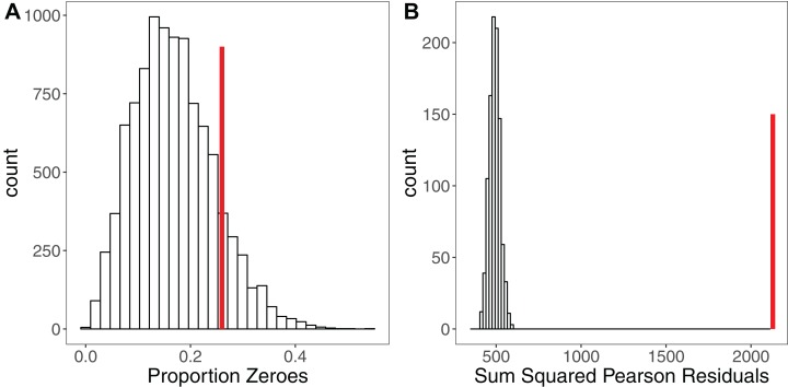
“Controlling for overdispersion in counts through the use of a glmm with an observation-level random effect (Harrison et al., 2018) fixed the problem of inflated type I error rates for distributions D2 and D7 (Fig. 3, indicated in red)”
From Violating the normality assumption may be the lesser of two evils (2021) · cites this paper as Harrison et al., 2018
In the citing paper
“Furthermore, as data were unbalanced, the use of a linear mixed model with different levels of correlations was necessary.42 This allowed all data to be used, and by including participant as a random effect, it ensured that each participant had their own baseline level, and the estimated change from baseline to visit 5 can be interpreted as the mean change from this level.”
From Increased Time in Range and Fewer Missed Bolus Injections After Introduction of a Smart Connected Insulin Pen (2020) · cites this paper as [42]
Self-check
Percentages, sums and reported differences re-computed from the paper’s own numbers.
The self-check needs the paper’s full text.
Citations
Cites
R: A Language and Environment for Statistical Computing
R Core Team (2000) · doi:10.32614/r.manuals · Cited by 355,893
Fitting Linear Mixed-Effects Models Using lme4
Bates, D., Mächler, M., Bolker, B., & Walker, S. (2015) · Journal of Statistical Software · doi:10.18637/jss.v067.i01 · Cited by 86,835
Model selection and multimodel inference: a practical information-theoretic approach.
Guthery, F. S., Burnham, K. P., & Anderson, D. R. (2003) · The Journal of Wildlife Management · doi:10.2307/3802723 · Cited by 41,495
Mixed effects models and extensions in ecology with R
Zuur, A. F., Ieno, E. N., Walker, N., Saveliev, A. A., & Smith, G. M. (2009) · Statistics for Biology and Health · doi:10.1007/978-0-387-87458-6 · Cited by 17,963
Multimodel Inference: Understanding AIC and BIC in Model Selection
Burnham, K. P., & Anderson, D. R. (2004) · Sociological Methods & Research · doi:10.1177/0049124104268644 · Cited by 11,648
Experimental Design and Data Analysis for Biologists
Quinn, G. P., & Keough, M. J. (2002) · doi:10.1017/cbo9780511806384 · Cited by 10,674 · cited 1×
“…parameters to be estimated can result in overparameterised models, where there are insufficient data to estimate coefficients robustly (Southwood & Henderson 2000, Quinn & Keough 2002, Crawley 2013 expected fitted lines of a 3-way interaction means refraining from fitting a model containing one.”
BackgroundA general and simple method for obtaining R 2 from generalized linear mixed‐effects models
Nakagawa, S., & Schielzeth, H. (2013) · Methods in Ecology and Evolution · doi:10.1111/j.2041-210x.2012.00261.x · Cited by 10,356
Random effects structure for confirmatory hypothesis testing: Keep it maximal
Barr, D. J., Levy, R., Scheepers, C., & Tily, H. J. (2013) · Journal of Memory and Language · doi:10.1016/j.jml.2012.11.001 · Cited by 10,328
Dormann, C. F., Elith, J., Bacher, S., Buchmann, C., Carl, G., Carré, G., Marquéz, J. R. G., Gruber, B., Lafourcade, B., Leitão, P. J., et al. (2013) · Ecography · doi:10.1111/j.1600-0587.2012.07348.x · Cited by 9,998
Generalized linear mixed models: a practical guide for ecology and evolution
Bolker, B. M., Brooks, M. E., Clark, C. J., Geange, S. W., Poulsen, J. R., Stevens, M. H. H., & White, J.-S. S. (2009) · Trends in Ecology & Evolution · doi:10.1016/j.tree.2008.10.008 · Cited by 8,910
Research works printed but not linked: 5
- Cox, 1989, The Analysis of Binary Data
- Crawley, 2013, The R Book
- Noble, 2017, Planned missing data design: stronger inferences increased research efficiency and improved animal welfare in ecology and evolution, bioRxiv, 247064, 10.1101/247064 · DOI
- Peters, 1991, A Critique for Ecology
- Southwood, 2000, Ecological Methods
Cited by
Sorted by citations
Robustness of linear mixed-effects models to violations of distributional assumptions
Schielzeth, H., Dingemanse, N. J., Nakagawa, S., Westneat, D. F., Allegue, H., Teplitsky, C., Réale, D., Dochtermann, N. A., Garamszegi, L. Z., & Araya‐Ajoy, Y. G. (2020) · Methods in Ecology and Evolution · doi:10.1111/2041-210x.13434 · Cited by 1,393
O’Dea, R. E., Lagisz, M., Jennions, M. D., Koricheva, J., Noble, D. W. A., Parker, T. H., Gurevitch, J., Page, M. J., Stewart, G. B., Moher, D., et al. (2021) · Biological reviews/Biological reviews of the Cambridge Philosophical Society · doi:10.1111/brv.12721 · Cited by 825
Violating the normality assumption may be the lesser of two evils
Knief, U., & Forstmeier, W. (2021) · Behavior Research Methods · doi:10.3758/s13428-021-01587-5 · Cited by 654
Lai, J., Zou, Y., Zhang, S., Zhang, X., & Mao, L. (2022) · Journal of Plant Ecology · doi:10.1093/jpe/rtac096 · Cited by 565
Estimating power in (generalized) linear mixed models: An open introduction and tutorial in R
Kumle, L., Võ, M. L.-H., & Draschkow, D. (2021) · Behavior Research Methods · doi:10.3758/s13428-021-01546-0 · Cited by 552
Climate-change-driven growth decline of European beech forests
del Castillo, E. M., Zang, C. S., Buras, A., Hacket-Pain, A., Esper, J., Serrano-Notivoli, R., Hartl, C., Weigel, R. F. B., Klesse, S., de Dios, V. R., et al. (2022) · Communications Biology · doi:10.1038/s42003-022-03107-3 · Cited by 274
Tapping into non-English-language science for the conservation of global biodiversity
Amano, T., Berdejo‐Espinola, V., Christie, A. P., Willott, K., Akasaka, M., Báldí, A., Berthinussen, A., Bertolino, S., Bladon, A. J., Chen, M., et al. (2021) · PLoS Biology · doi:10.1371/journal.pbio.3001296 · Cited by 270
Ignoring non‐English‐language studies may bias ecological meta‐analyses
Konno, K., Akasaka, M., Koshida, C., Katayama, N., Osada, N., Spake, R., & Amano, T. (2020) · Ecology and Evolution · doi:10.1002/ece3.6368 · Cited by 260
Tracking the global reduction of marine traffic during the COVID-19 pandemic
March, D., Metcalfe, K., Tintoré, J., & Godley, B. J. (2021) · Nature Communications · doi:10.1038/s41467-021-22423-6 · Cited by 240
Online teaching self-efficacy during COVID-19: Changes, its associated factors and moderators
Ma, K., Chutiyami, M., Zhang, Y., & Nicoll, S. (2021) · Education and Information Technologies · doi:10.1007/s10639-021-10486-3 · Cited by 218
Fisher, J. C., Irvine, K. N., Bicknell, J. E., Hayes, W. M., Fernandes, D., Mistry, J., & Davies, Z. G. (2020) · The Science of The Total Environment · doi:10.1016/j.scitotenv.2020.143095 · Cited by 233
Predicting lapses of attention with sleep-like slow waves
Andrillon, T., Burns, A. C., Mackay, T., Windt, J., & Tsuchiya, N. (2021) · Nature Communications · doi:10.1038/s41467-021-23890-7 · Cited by 236
Leroux, S. (2019) · PLoS ONE · doi:10.1371/journal.pone.0206711 · Cited by 192
Linking green infrastructure to urban heat and human health risk mitigation in Oslo, Norway
Venter, Z. S., Krog, N. H., & Barton, D. N. (2020) · Science of The Total Environment · doi:10.1016/j.scitotenv.2019.136193 · Cited by 191
Brownscombe, J. W., Lédée, E. J. I., Raby, G. D., Struthers, D. P., Gutowsky, L. F. G., Nguyen, V. M., Young, N., Stokesbury, M. J. W., Holbrook, C. M., Brenden, T. O., et al. (2019) · Reviews in Fish Biology and Fisheries · doi:10.1007/s11160-019-09560-4 · Cited by 185
Rider, O. J., Apps, A. P., Miller, J. J. J. J., Lau, J. Y. C., Lewis, A., Peterzan, M. A., Dodd, M. S., Lau, A. Z., Trumper, C., Gallagher, F. A., et al. (2020) · Circulation Research · doi:10.1161/circresaha.119.316260 · Cited by 172
Mokany, K., Ware, C., Woolley, S. N. C., Ferrier, S., & Fitzpatrick, M. C. (2022) · Global Ecology and Biogeography · doi:10.1111/geb.13459 · Cited by 172
Morris, S. D., Brook, B. W., Moseby, K. E., & Johnson, C. N. (2021) · Global Ecology and Conservation · doi:10.1016/j.gecco.2021.e01630 · Cited by 164
Frontiers in quantifying wildlife behavioural responses to chemical pollution
Bertram, M. G., Martin, J. M., McCallum, E. S., Alton, L. A., Brand, J. A., Brooks, B. W., Červený, D., Fick, J. B., Ford, A. T., Hellström, G., et al. (2022) · Biological reviews/Biological reviews of the Cambridge Philosophical Society · doi:10.1111/brv.12844 · Cited by 172
Tree planting in organic soils does not result in net carbon sequestration on decadal timescales
Friggens, N. L., Hester, A. J., Mitchell, R. J., Parker, T. C., Subke, J., & Wookey, P. A. (2020) · Global Change Biology · doi:10.1111/gcb.15229 · Cited by 168
A translucent box: interpretable machine learning in ecology
Lucas, T. C. D. (2020) · Ecological Monographs · doi:10.1002/ecm.1422 · Cited by 161
Gomes, D. G. E. (2022) · PeerJ · doi:10.7717/peerj.12794 · Cited by 169
Merritt, K., McGuire, P. K., Egerton, A., 1H-MRS in Schizophrenia Investigators, Aleman, A., Block, W., Bloemen, O., Borgan, F., Bustillo, J., Capizzano, A. A., et al. (2021) · JAMA Psychiatry · doi:10.1001/jamapsychiatry.2021.0380 · Cited by 142
Adolfsson, P., Hartvig, N. V., Kaas, A., Møller, J. B., & Hellman, J. (2020) · Diabetes Technology & Therapeutics · doi:10.1089/dia.2019.0411 · Cited by 139
Mixed Models Offer No Freedom from Degrees of Freedom
Arnqvist, G. (2020) · Trends in Ecology & Evolution · doi:10.1016/j.tree.2019.12.004 · Cited by 135
Rates and drivers of aboveground carbon accumulation in global monoculture plantation forests
Bukoski, J. J., Cook‐Patton, S. C., Melikov, C., Ban, H., Chen, J. L., Goldman, E. D., Harris, N. L., & Potts, M. D. (2022) · Nature Communications · doi:10.1038/s41467-022-31380-7 · Cited by 150
Prevention not cure: a review of methods to avoid sea lice infestations in salmon aquaculture
Barrett, L. T., Oppedal, F., Robinson, N. A., & Dempster, T. (2020) · Reviews in Aquaculture · doi:10.1111/raq.12456 · Cited by 131
Physical activity and motor skills in children: A differentiated approach
Dapp, L. C., Gashaj, V., & Roebers, C. M. (2021) · Psychology of sport and exercise · doi:10.1016/j.psychsport.2021.101916 · Cited by 170
Kirtley, O. J., Lafit, G., Achterhof, R., Hiekkaranta, A. P., & Myin‐Germeys, I. (2021) · Advances in Methods and Practices in Psychological Science · doi:10.1177/2515245920924686 · Cited by 146
Not so robust: Robusta coffee production is highly sensitive to temperature
Kath, J. M., Byrareddy, V. M., Craparo, A., Nguyen‐Huy, T., Mushtaq, S., Cao, L., & Bossolasco, L. (2020) · Global Change Biology · doi:10.1111/gcb.15097 · Cited by 129
Continent-wide effects of urbanization on bird and mammal genetic diversity
Schmidt, C., Domaratzki, M., Kinnunen, R. P., Bowman, J., & Garroway, C. J. (2020) · Proceedings of the Royal Society B Biological Sciences · doi:10.1098/rspb.2019.2497 · Cited by 121
Optimum growth temperature declines with body size within fish species
Lindmark, M., Ohlberger, J., & Gårdmark, A. (2022) · Global Change Biology · doi:10.1111/gcb.16067 · Cited by 121
Temperature Controls eDNA Persistence across Physicochemical Conditions in Seawater
McCartin, L. J., Vohsen, S. A., Ambrose, S. W., Layden, M. J., McFadden, C. S., Cordes, E. E., McDermott, J. M., & Herrera, S. (2022) · Environmental Science & Technology · doi:10.1021/acs.est.2c01672 · Cited by 122
Human perturbations reduce dung beetle diversity and dung removal ecosystem function
Noriega, J. A., March‐Salas, M., Castillo, S., García-Q., H., Hortal, J., & Santos, A. M. C. (2021) · Biotropica · doi:10.1111/btp.12953 · Cited by 115
Temperature and rainfall impacts on robusta coffee bean characteristics
Kath, J. M., Byrareddy, V. M., Mushtaq, S., Craparo, A., & Porcel, M. (2021) · Climate Risk Management · doi:10.1016/j.crm.2021.100281 · Cited by 120
Pellegrini, A. F. A., Hobbie, S. E., Reich, P. B., Jumpponen, A., Brookshire, E. N. J., Caprio, A. C., Coetsee, C., & Jackson, R. B. (2020) · Ecological Monographs · doi:10.1002/ecm.1409 · Cited by 121
Massoni, J., Bortfeld‐Miller, M., Jardillier, L. E., Salazar, G., Sunagawa, S., & Vorholt, J. A. (2019) · The ISME Journal · doi:10.1038/s41396-019-0531-8 · Cited by 106
Oberpriller, J., Leite, M. D. S., & Pichler, M. (2022) · Ecology and Evolution · doi:10.1002/ece3.9062 · Cited by 105
Nutrients and not temperature are the key drivers for cyanobacterial biomass in the Americas
Bonilla, S., Aguilera, A., Aubriot, L., Huszar, V. L. M., Almanza, V., Haakonsson, S., Izaguirre, I., O’Farrell, I., Salazar-Torres, A., Becker, V., et al. (2022) · Harmful Algae · doi:10.1016/j.hal.2022.102367 · Cited by 104
Palencia, P., Vicente, J., Soriguer, R. C., & Acevedo, P. (2021) · Journal of Zoology · doi:10.1111/jzo.12945 · Cited by 101
Continental-scale controls on soil organic carbon across sub-Saharan Africa
von Fromm, S. F., Hoyt, A. M., Acquah, G., Aynekulu, E., Berhe, A. A., Haefele, S. M., Lange, M., McGrath, S. P., Shepherd, K. D., Sila, A., et al. (2021) · SOIL · doi:10.5194/soil-7-305-2021 · Cited by 106
Seventy years of tunas, billfishes, and sharks as sentinels of global ocean health
Juan‐Jordá, M. J., Murua, H., Arrizabalaga, H., Merino, G., Pacoureau, N., & Dulvy, N. K. (2022) · Science · doi:10.1126/science.abj0211 · Cited by 99
Perils and pitfalls of mixed-effects regression models in biology
Silk, M. J., Harrison, X. A., & Hodgson, D. J. (2020) · PeerJ · doi:10.7717/peerj.9522 · Cited by 98
Self-citationJones, G. M., Kramer, H. A., Whitmore, S. A., Berigan, W. J., Tempel, D. J., Wood, C. M., Hobart, B. K., Erker, T., Atuo, F. A., Pietrunti, N. F., et al. (2020) · Landscape Ecology · doi:10.1007/s10980-020-01010-y · Cited by 93
Differential cooling effects of landscape parameters in humid-subtropical urban parks
Cheung, P. K., & Jim, C. Y. (2019) · Landscape and Urban Planning · doi:10.1016/j.landurbplan.2019.103651 · Cited by 97
Local‐scale climatic refugia offer sanctuary for a habitat‐forming species during a marine heatwave
Verdura, J., Santamaría, J., Ballesteros, E., Smale, D. A., Cefalì, M. E., Golo, R., de Caralt, S., Vergés, A., & Cebrián, E. (2021) · Journal of Ecology · doi:10.1111/1365-2745.13599 · Cited by 101
Airfoil-like mechanics generate thrust on the anterior body of swimming fishes
Lucas, K. N., LAUDER, G. V., & Tytell, E. D. (2020) · Proceedings of the National Academy of Sciences · doi:10.1073/pnas.1919055117 · Cited by 97
Causal Inference With Observational Data and Unobserved Confounding Variables
Byrnes, J. E. K., & Dee, L. E. (2025) · Ecology Letters · doi:10.1111/ele.70023 · Cited by 111
Temperate agroforestry systems provide greater pollination service than monoculture
Varah, A., Jones, H., Smith, J., & Potts, S. G. (2020) · Agriculture Ecosystems & Environment · doi:10.1016/j.agee.2020.107031 · Cited by 89
A global baseline for qPCR-determined antimicrobial resistance gene prevalence across environments
Abramova, A., Berendonk, T. U., & Bengtsson‐Palme, J. (2023) · Environment International · doi:10.1016/j.envint.2023.108084 · Cited by 89
Harrison, X. A., Price, S. J., Hopkins, K., Leung, W. T. M., Sergeant, C., & Garner, T. W. J. (2019) · Frontiers in Microbiology · doi:10.3389/fmicb.2019.02883 · Cited by 88
Self-citationSocial bonds provide multiple pathways to reproductive success in wild male chimpanzees
Feldblum, J. T., Krupenye, C., Bray, J., Pusey, A. E., & Gilby, I. C. (2021) · iScience · doi:10.1016/j.isci.2021.102864 · Cited by 87
Salmela‐Aro, K., Upadyaya, K., Ronkainen, I., & Hietajärvi, L. (2022) · Journal of Happiness Studies · doi:10.1007/s10902-022-00518-1 · Cited by 137
Beaumelle, L., Auriol, A., Grasset, M., Pavy, A., Thiéry, D., & Rusch, A. (2021) · Ecological Solutions and Evidence · doi:10.1002/2688-8319.12086 · Cited by 106
Sorek‐Hamer, M., Chatfield, R. B., & Liu, Y. (2020) · Environment International · doi:10.1016/j.envint.2020.106057 · Cited by 83
Decadal changes in fire frequencies shift tree communities and functional traits
Pellegrini, A. F. A., Refsland, T. K., Averill, C., Terrer, C., Staver, A. C., Brockway, D. G., Caprio, A. C., Clatterbuck, W. K., Coetsee, C., Haywood, J. D., et al. (2021) · Nature Ecology & Evolution · doi:10.1038/s41559-021-01401-7 · Cited by 87
A meta-analysis reveals edge effects within marine protected areas
Ohayon, S., Granot, I., & Belmaker, J. (2021) · Nature Ecology & Evolution · doi:10.1038/s41559-021-01502-3 · Cited by 78
Reward-Based Improvements in Motor Control Are Driven by Multiple Error-Reducing Mechanisms
Codol, O., Holland, P. J., Manohar, S., & Galea, J. M. (2020) · Journal of Neuroscience · doi:10.1523/jneurosci.2646-19.2020 · Cited by 73
Environmental heterogeneity dynamics drive plant diversity on oceanic islands
Barbosa, M. P. B., Weigelt, P., Borregaard, M. K., Keppel, G., & Kreft, H. (2020) · Journal of Biogeography · doi:10.1111/jbi.13925 · Cited by 76
He, P., Shi, L., Li, Y., Duan, Q., Qiu, Y., Feng, S., Gao, Y., Luo, Y., Ma, G., Zhang, Y., et al. (2023) · Annals of Neurology · doi:10.1002/ana.26729 · Cited by 77
Age influences domestic dog cognitive performance independent of average breed lifespan
Watowich, M. M., MacLean, E. L., Hare, B. A., Call, J., Kaminski, J., Miklósi, Á., & Snyder‐Mackler, N. (2020) · Animal Cognition · doi:10.1007/s10071-020-01385-0 · Cited by 80
Lim, J. Y., Svenning, J., Göldel, B., Faurby, S., & Kissling, W. D. (2020) · Nature Communications · doi:10.1038/s41467-020-18530-5 · Cited by 75
Quantifying crop pollinator dependence and its heterogeneity using multi‐level meta‐analysis
Bishop, J., & Nakagawa, S. (2020) · Journal of Applied Ecology · doi:10.1111/1365-2664.13830 · Cited by 76
Chanyalew, M. A., Yitayal, M., Atnafu, A., & Tilahun, B. C. (2021) · BMC Medical Informatics and Decision Making · doi:10.1186/s12911-021-01400-5 · Cited by 75
Xiang, W., Li, L., Ouyang, S., Xiao, W., Zeng, L., Chen, L., Lei, P., Deng, X., Zeng, Y., Fang, J., et al. (2020) · European Journal of Forest Research · doi:10.1007/s10342-020-01333-0 · Cited by 74
Dealing with small samples in football research
Hecksteden, A., Kellner, R., & Donath, L. (2021) · Science and Medicine in Football · doi:10.1080/24733938.2021.1978106 · Cited by 74
Kath, J. M., Craparo, A., Fong, Y., Byrareddy, V. M., Davis, A. P., King, R., Nguyen‐Huy, T., van Asten, P., Marcussen, T., Mushtaq, S., et al. (2022) · Nature Food · doi:10.1038/s43016-022-00614-8 · Cited by 85
Hot droughts compromise interannual survival across all group sizes in a cooperatively breeding bird
Bourne, A. R., Cunningham, S. J., Spottiswoode, C. N., & Ridley, A. R. (2020) · Ecology Letters · doi:10.1111/ele.13604 · Cited by 84
Hydrolyzable microplastics in soil—low biodegradation but formation of a specific microbial habitat?
Schöpfer, L., Schnepf, U., Marhan, S., Brümmer, F., Kandeler, E., & Pagel, H. (2022) · Biology and Fertility of Soils · doi:10.1007/s00374-022-01638-9 · Cited by 75
Global meta-analysis shows reduced quality of food crops under inadequate animal pollination
Gazzea, E., Batáry, P., & Marini, L. (2023) · Nature Communications · doi:10.1038/s41467-023-40231-y · Cited by 82
Migraine attacks as a result of hypothalamic loss of control
Stankewitz, A., Keidel, L., Rehm, M., Irving, S., Kaczmarz, S., Preibisch, C., Witkovský, V., Zimmer, C., Schulz, E., & Toelle, T. (2020) · bioRxiv · doi:10.1016/j.nicl.2021.102784 · Cited by 61
Schindler, T., Mander, Ü., Macháčová, K., Espenberg, M., Krasnov, D., Escuer-Gatius, J., Veber, G., Pärn, J., & Soosaar, K. (2020) · Scientific Reports · doi:10.1038/s41598-020-60058-7 · Cited by 69
Negative binomial mixed models for analyzing longitudinal CD4 count data
Yirga, A. A., Melesse, S. F., Mwambi, H. G., & Ayele, D. G. (2020) · Scientific Reports · doi:10.1038/s41598-020-73883-7 · Cited by 69
Franklin, A. M., Weller, D. L., Durso, L. M., Bagley, M. J., Davis, B. C., Frye, J. G., Grim, C. J., Ibekwe, A. M., Jahne, M. A., Keely, S. P., et al. (2024) · Frontiers in Water · doi:10.3389/frwa.2024.1359109 · Cited by 73
Tulbure, M. G., & Broich, M. (2018) · The Science of The Total Environment · doi:10.1016/j.scitotenv.2018.11.390 · Cited by 70
Yuan, H., Liang, J., Lin, P., Sucipto, K., Tsegaye, M. M., Wen, T., Pfeiffer, S., & Pfeiffer, D. U. (2020) · Scientific Reports · doi:10.1038/s41598-020-60309-7 · Cited by 68
Burdine, J. D., & McCluney, K. E. (2019) · Oecologia · doi:10.1007/s00442-019-04416-x · Cited by 67
Sex‐specific effects of wind on the flight decisions of a sexually dimorphic soaring bird
Clay, T. A., Joo, R., Weimerskirch, H., Phillips, R. A., den Ouden, O. F. C., Basille, M., Clusella‐Trullas, S., Assink, J. D., & Patrick, S. C. (2020) · Journal of Animal Ecology · doi:10.1111/1365-2656.13267 · Cited by 73
High temperatures drive offspring mortality in a cooperatively breeding bird
Bourne, A. R., Cunningham, S. J., Spottiswoode, C. N., & Ridley, A. R. (2020) · Proceedings of the Royal Society B Biological Sciences · doi:10.1098/rspb.2020.1140 · Cited by 67
The influence of landscape composition and configuration on crop yield resilience
Redhead, J. W., Oliver, T. H., Woodcock, B. A., & Pywell, R. F. (2020) · Journal of Applied Ecology · doi:10.1111/1365-2664.13722 · Cited by 73
Guo, Y., Abdalla, M., Espenberg, M., Hastings, A., Hallett, P. D., & Smith, P. (2020) · The Science of The Total Environment · doi:10.1016/j.scitotenv.2020.143824 · Cited by 67
Cattle don’t care: Animal behaviour is similar regardless of grazing management in grasslands
Venter, Z. S., Hawkins, H., & Cramer, M. D. (2018) · Agriculture Ecosystems & Environment · doi:10.1016/j.agee.2018.11.023 · Cited by 66
Coping with climate change: limited behavioral responses to hot weather in a tropical carnivore
Rabaiotti, D., & Woodroffe, R. (2019) · Oecologia · doi:10.1007/s00442-018-04329-1 · Cited by 70
Violating the normality assumption may be the lesser of two evilsPreprint
Knief, U., & Forstmeier, W. (2018) · bioRxiv (Cold Spring Harbor Laboratory) · doi:10.1101/498931 · Cited by 67
Braga‐Pereira, F., Morcatty, T. Q., Bizri, H. R. E., Tavares, A. S., Roncal, C. M., González‐Crespo, C., Bertsch, C., Rodriguez, C. R., Bardales‐Alvites, C., von Mühlen, E. M., et al. (2021) · Methods in Ecology and Evolution · doi:10.1111/2041-210x.13773 · Cited by 64
The consequences of checking for zero‐inflation and overdispersion in the analysis of count data
Campbell, H. (2021) · Methods in Ecology and Evolution · doi:10.1111/2041-210x.13559 · Cited by 71
Ecological Correlates of Elevational Range Shifts in Tropical Birds
Neate‐Clegg, M. H. C., Jones, S. E. I., Tobias, J. A., Newmark, W. D., & Şekercioğlu, Ç. H. (2021) · Frontiers in Ecology and Evolution · doi:10.3389/fevo.2021.621749 · Cited by 66
Htay, T., Htoo, K. K., Mbise, F. P., & Røskaft, E. (2022) · Society & Natural Resources · doi:10.1080/08941920.2022.2032515 · Cited by 62
Dwarfism and gigantism drive human-mediated extinctions on islands
Rozzi, R., Lomolino, M. V., van der Geer, A. A. E., Silvestro, D., Lyons, S. K., Bover, P. R., Alcover, J. A., Benítez‐López, A., Tsai, C., Fujita, M., et al. (2023) · Science · doi:10.1126/science.add8606 · Cited by 66
Judgements of a speaker’s personality are correlated across differing content and stimulus type
Mahrholz, G., Belin, P., & McAleer, P. (2018) · PLoS ONE · doi:10.1371/journal.pone.0204991 · Cited by 61
Pangolins in global camera trap data: Implications for ecological monitoring
Khwaja, H., Buchan, C., Wearn, O. R., Bahaa‐el‐din, L., Bantlin, D. A., Bernard, H., Bitariho, R., Bohm, T., Borah, J., Brodie, J. F., et al. (2019) · Global Ecology and Conservation · doi:10.1016/j.gecco.2019.e00769 · Cited by 62
van den Dries, M. A., Guxens, M., Pronk, A., Spaan, S., Marroun, H. E., Jusko, T. A., Longnecker, M. P., Ferguson, K. K., & Tiemeier, H. W. (2019) · Environment International · doi:10.1016/j.envint.2019.105002 · Cited by 65
Surana, B., Ferre, C. L., Dew, A. P., Brandão, M. B., Gordon, A. M., & Moreau, N. G. (2019) · Neurorehabilitation and neural repair · doi:10.1177/1545968319868719 · Cited by 65
Association of food insecurity with MASLD prevalence and liver-related mortality
Younossi, Z. M., Zelber‐Sagi, S., Kugelmas, C., Lazarus, J. V., Paik, A., de Avila, L., Gerber, L. H., & Paik, J. M. (2024) · Journal of Hepatology · doi:10.1016/j.jhep.2024.08.011 · Cited by 60
On the indeterministic nature of star formation on the cloud scale
Geen, S., Watson, S. K., Rosdahl, J., Bieri, R., Klessen, R. S., & Hennebelle, P. (2018) · Monthly Notices of the Royal Astronomical Society · doi:10.1093/mnras/sty2439 · Cited by 59
Allen, L. C., Hristov, N. I., Rubin, J. J., Lightsey, J. T., & Barber, J. R. (2021) · Proceedings of the Royal Society B Biological Sciences · doi:10.1098/rspb.2020.2689 · Cited by 59
Teich, M., Giunta, A. D., Hagenmuller, P., Bebi, P., Schneebeli, M., & Jenkins, M. J. (2019) · Forest Ecology and Management · doi:10.1016/j.foreco.2019.01.052 · Cited by 58
Urban food subsidies reduce natural food limitations and reproductive costs for a wetland bird
Evans, B. A., & Gawlik, D. E. (2020) · Scientific Reports · doi:10.1038/s41598-020-70934-x · Cited by 57
Shibabaw, T., Beyene, A., Awoke, A., Bayih, M. T., Azage, M., & Triest, L. (2021) · PLoS ONE · doi:10.1371/journal.pone.0246043 · Cited by 68
Revealing the hidden carbon in forested wetland soils
Stewart, A. J., Halabisky, M. A., Babcock, C., Butman, D., D’Amore, D. V., & Moskal, L. M. (2024) · Nature Communications · doi:10.1038/s41467-024-44888-x · Cited by 58
Metadata
- Authors
- Harrison, X. A., Donaldson, L., Correa-Cano, M. E., Evans, J., Fisher, D. N., Goodwin, C. E. D., Robinson, B. S., Hodgson, D. J., & Inger, R.
- Affiliations
- Zoological Society of London (GB)
- University of Exeter (GB)
- Environment and Sustainability Institute, University of Exeter, Penryn, UK
- University of Ottawa (CA)
- Corresponding author
- Harrison, Xavier A.
- ORCID
- Venue
- PeerJ
- Publisher
- PeerJ
- Published
- 2018-05-23
- Volume
- 6
- Pages
- e4794
- ISSN
- 2167-8359 (ISSN-L)
- PMC
- PMC5970551
- OpenAlex
- W2783564415
- Cited by
- 2,094
- References
- 91
- Citations by year
- 2026: 227 · 2025: 228 · 2024: 271 · 2023: 246 · 2022: 327 · 2021: 383 · 2020: 261 · 2019: 116 · 2018: 32
- FWCI
- 164.31
- Type
- journal article
- Language
- en
- Open access
- gold
- doi.org
- Locations
- PeerJ (publishedVersion, cc-by)
- Europe PMC (PubMed Central) (publishedVersion, cc-by)
- PubMed Central (publishedVersion, cc-by)
- PubMed (publishedVersion)
- Aberdeen University Research Archive (Aberdeen University) (submittedVersion)
- DOAJ (DOAJ: Directory of Open Access Journals) (submittedVersion, cc-by-sa)
- Funders
- Institute of Zoology Research Fellowship
- NERC studentship (NE/H02249X/1, NE/L501669/1)
- University of Exeter and the Animal and Plant Health as part of ‘Wildlife Research Co-Operative’
- CONACYT (The Mexican National Council for Science and Technology)
- SEP (The Mexican Ministry of Education)
- Forestry Commission
- Topics
- Physical Sciences › Mathematics › Statistics and Probability › Statistical Methods and Bayesian Inference
- Life Sciences › Agricultural and Biological Sciences › Agronomy and Crop Science › Agriculture, Soil, Plant Science
- Physical Sciences › Mathematics › Statistics and Probability › Statistical Methods and Applications
- Keywords
- linear mixed models, multi-model inference, model selection, information theory, ecological data analysis, statistical pitfalls
About these checks
Registry, retraction, Cites and statistics results are computed, not judged, with one exception: a printed reference that no index lists is read once by a model before it counts as a citation error. Claims are extracted by a model and kept only when their quote appears verbatim in the text; each cited source is then checked, with a model’s help, for whether it says what the claim relies on. Those verdicts can be wrong — read the claim’s quote and the cited source before relying on one.
Statistics and arithmetic are recomputed, not judged.
Confidence bands are shown only for fields calibrated on our annotated test set. None is calibrated yet, so no band is shown.
What counts as a claim ›How we measure confidence ›How we check this ›
Are you an author, or do you see a problem with this page? Request a review
