

The DOI matches its Crossref record; 6 of the 6 references it cites were found in a registry or an index.
Predictive performance of presence‐only species distribution models: a benchmark study with reproducible code
Abstract
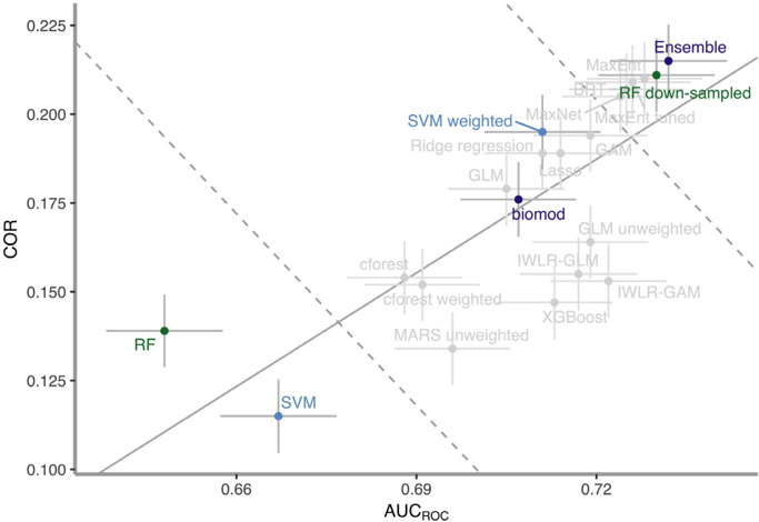
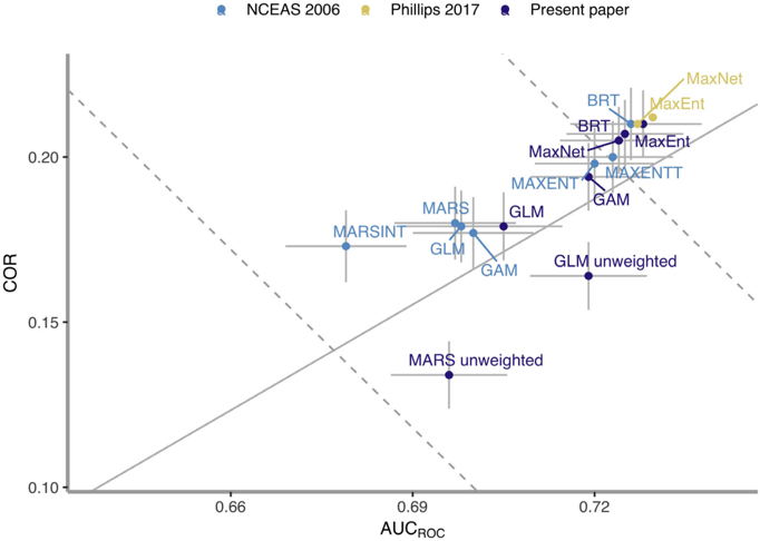
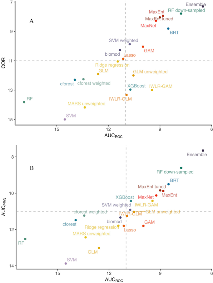
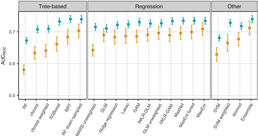
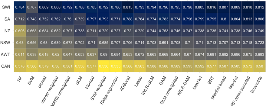
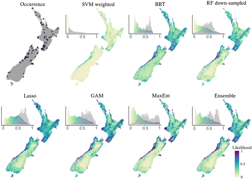
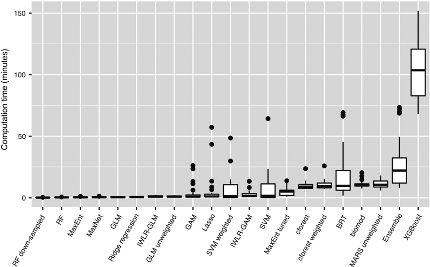
Species distribution modeling (SDM) is widely used in ecology and conservation. Currently, the most available data for SDM are species presence‐only records (available through digital databases). There have been many studies comparing the performance of alternative algorithms for modeling presence‐only data. Among these, a 2006 paper from Elith and colleagues has been particularly influential in the field, partly because they used several novel methods (at the time) on a global data set that included independent presence–absence records for model evaluation. Since its publication, some of the algorithms have been further developed and new ones have emerged. In this paper, we explore patterns in predictive performance across methods, by reanalyzing the same data set (225 species from six different regions) using updated modeling knowledge and practices. We apply well‐established methods such as generalized additive models and MaxEnt, alongside others that have received attention more recently, including regularized regressions, point‐process weighted regressions, random forests, XGBoost, support vector machines, and the ensemble modeling framework biomod. All the methods we use include background samples (a sample of environments in the landscape) for model fitting. We explore impacts of using weights on the presence and background points in model fitting. We introduce new ways of evaluating models fitted to these data, using the area under the precision‐recall gain curve, and focusing on the rank of results. We find that the way models are fitted matters. The top method was an ensemble of tuned individual models. In contrast, ensembles built using the biomod framework with default parameters performed no better than single moderate performing models. Similarly, the second top performing method was a random forest parameterized to deal with many background samples (contrasted to relatively few presence records), which substantially outperformed other random forest implementations. We find that, in general, nonparametric techniques with the capability of controlling for model complexity outperformed traditional regression methods, with MaxEnt and boosted regression trees still among the top performing models. All the data and code with working examples are provided to make this study fully reproducible.
Overview
The claims and statistics of this paper haven’t been checked yet.
Run the check — free, no account needed. It reads the open-access text and checks the sources it cites.
Integrity signals
Registry
Cites
Statistics
Figures
Verification
Claims the paper makes
The claims and statistics of this paper haven’t been checked yet.
Run the check — free, no account needed. It reads the open-access text and checks the sources it cites.
Claims other papers make about this one
Each is checked against this paper’s own text: does it say what the citing paper says it does?
The source backs part of the claim, not all of it — or backs it for a different population, condition or comparison.
In the citing paper
“It has been recognized for its efficiency and effectiveness in handling large and complex datasets across various domains, including SDM (Valavi et al., 2022).”
From Predictive modeling for targeted archaeological survey of arsacid period sites in the iranian borderland region of the araxes river valley (2026) · cites this paper as Valavi et al., 2022
Experimental — accuracy not yet measured
Self-check
Percentages, sums and reported differences re-computed from the paper’s own numbers.
The self-check needs the paper’s full text.
Citations
Cites
XGBoost: A Scalable Tree Boosting System
Chen, T., & Guestrin, C. (2016) · Proceedings of the 22nd ACM SIGKDD International Conference on Knowledge Discovery and Data Mining · doi:10.1145/2939672.2939785 · Cited by 54,569
Model selection and multimodel inference: a practical information-theoretic approach.
Guthery, F. S., Burnham, K. P., & Anderson, D. R. (2003) · The Journal of Wildlife Management · doi:10.2307/3802723 · Cited by 41,495
Kuhn, M., & Johnson, K. (2013) · doi:10.1007/978-1-4614-6849-3 · Cited by 6,788
Saito, T., & Rehmsmeier, M. (2015) · PLOS ONE · doi:10.1371/journal.pone.0118432 · Cited by 5,309
Unbiased Recursive Partitioning: A Conditional Inference Framework
Hothorn, T., Hornik, K., & Zeileis, A. (2006) · Journal of Computational and Graphical Statistics · doi:10.1198/106186006x133933 · Cited by 4,021
Strobl, C., Malley, J., & Tutz, G. (2009) · Psychological Methods · doi:10.1037/a0016973 · Cited by 2,583
Research works printed but not linked: 120
- 10.1007/978-3-540-30115-8_7 · DOI
- Ali A., 2015, Classification with class imbalance problem: a review, International Journal of Advances in Soft Computing and Its Applications, 7, 176
- 10.1111/j.1365-2664.2006.01214.x · DOI · Paper page
- 10.1111/j.1749-6632.2011.06440.x · DOI
- 10.1126/sciadv.aat4858 · DOI
- 10.1016/j.tree.2006.09.010 · DOI · Paper page
- 10.1002/ecs2.1825 · DOI
- 10.1016/S0378-1127(96)03753-X · DOI
- 10.1111/j.1600-0706.2012.00299.x · DOI
- 10.1111/j.2041-210X.2011.00172.x · DOI · Paper page
- 10.1016/j.ecolmodel.2016.10.004 · DOI
- 10.1016/j.tree.2008.10.008 · DOI · Paper page
- 10.1111/ddi.12144 · DOI
- Boyd K., 2012, Unachievable region in precision‐recall space and its effect on empirical evaluation
- 10.1111/2041-210X.12957 · DOI
- 10.1111/geb.12102 · DOI
- 10.32614/RJ-2016-017 · DOI
- Chen C., 2004, Using random forest to learn imbalanced data, University of California, Berkeley
- 10.1093/biomet/45.3-4.562 · DOI · Paper page
- Demšar J., 2006, Statistical comparisons of classifiers over multiple data sets, Journal of Machine Learning Research, 7, 30
- 10.1126/science.aat7526 · DOI
- 10.1002/ecm.1309 · DOI
- 10.1111/j.1365-2664.2006.01141.x · DOI
- 10.1111/ecog.03149 · DOI
- 10.1111/j.2006.0906-7590.04596.x · DOI · Paper page
- Elith J., 2019, Quantitative analyses in wildlife science
- 10.17161/bi.v15i2.13384 · DOI
- 10.1111/j.1472-4642.2007.00340.x · DOI
- Elith J., 2009, Spatial conservation prioritization: quantitative methods, 70, 10.1093/oso/9780199547760.003.0006 · DOI · Paper page
- 10.1111/j.1365-2656.2008.01390.x · DOI · Paper page
- 10.1111/j.1472-4642.2010.00725.x · DOI · Paper page
- 10.1007/s10980-009-9341-0 · DOI
- Fidler F., 2017, Metaresearch for evaluating reproducibility in ecology and evolution, BioScience, 67, 282
- 10.1111/2041-210X.12242 · DOI
- 10.1214/13-AOAS667 · DOI
- Flach P., 2015, Advances in neural information processing systems, 838
- 10.1017/CBO9780511810602 · DOI
- 10.1139/cjfr-2014-0562 · DOI
- 10.1016/S0167-9473(01)00065-2 · DOI · Paper page
- 10.18637/jss.v033.i01 · DOI · Paper page
- 10.1016/j.ins.2009.12.010 · DOI
- García S., 2008, An extension on “statistical comparisons of classifiers over multiple data sets” for all pairwise comparisons, Journal of Machine Learning Research, 9, 2677
- 10.1016/j.ecolmodel.2011.04.015 · DOI
- 10.1111/geb.12268 · DOI
- 10.1111/ele.12189 · DOI
- 10.1111/j.1461-0248.2005.00792.x · DOI
- 10.1017/9781139028271 · DOI
- 10.1016/j.ecolmodel.2004.07.012 · DOI
- 10.1016/j.ecolmodel.2019.108719 · DOI
- 10.1111/ddi.12892 · DOI
- 10.1111/ecog.04890 · DOI
- 10.7717/peerj.4278 · DOI
- 10.1111/j.1600-0587.2013.00321.x · DOI
- 10.1007/978-0-387-84858-7 · DOI · Paper page
- 10.1109/TKDE.2008.239 · DOI · Paper page
- 10.1007/s40823-016-0008-7 · DOI
- Herdter E., 2019, Using extreme gradient boosting (XGBoost) to evaluate the importance of a suite of environmental variables and to predict recruitment of young‐of‐the‐year spotted seatrout in Florida, bioRxiv, 543181
- 10.1016/j.ecolmodel.2006.05.017 · DOI
- Huang H., 2018, FVID: Fishing vessel type identification based on VMS trajectories, Journal of Ocean University of China, 17, 1
- Hughes‐Oliver J. M., 2018, Population and empirical PR curves for assessment of ranking algorithms
- 10.1111/2041-210X.13496 · DOI
- 10.1007/978-1-4614-7138-7 · DOI · Paper page
- 10.3233/IDA-2002-6504 · DOI · Paper page
- 10.1109/CIDU.2012.6382186 · DOI
- 10.1016/j.ecolmodel.2019.108927 · DOI
- 10.1186/1472-6947-11-51 · DOI
- 10.1093/oxfordjournals.pan.a004868 · DOI · Paper page
- 10.1101/gr.092759.109 · DOI
- Kull M., 2019, Advances in Neural Information Processing Systems, 12295
- 10.1111/2041-210X.12123 · DOI · Paper page
- 10.1016/j.ecolmodel.2006.05.022 · DOI
- 10.1016/j.ecolmodel.2012.07.003 · DOI
- 10.1111/j.1472-4642.2008.00491.x · DOI
- 10.1016/j.csda.2011.02.004 · DOI
- 10.1111/ecog.00845 · DOI
- 10.1111/j.1365-2699.2007.01720.x · DOI
- 10.7717/peerj.2849 · DOI
- 10.1111/j.1749-8198.2010.00351.x · DOI
- 10.1016/j.ecoinf.2019.100974 · DOI
- 10.1111/2041-210X.12261 · DOI · Paper page
- 10.1111/cobi.13669 · DOI
- 10.1002/ecm.1370 · DOI
- 10.1016/S0304-3800(00)00322-7 · DOI
- 10.1111/j.1365-2699.2006.01460.x · DOI
- 10.1111/ecog.03049 · DOI · Paper page
- 10.1016/j.ecolmodel.2005.03.026 · DOI · Paper page
- 10.1111/j.0906-7590.2008.5203.x · DOI · Paper page
- 10.1890/07-2153.1 · DOI · Paper page
- 10.1890/09-0760.1 · DOI
- 10.1890/12-1520.1 · DOI
- Plummer M., 2003, Proceedings of the 3rd International Workshop on Distributed Statistical Computing, 1
- 10.1111/bij.12517 · DOI
- 10.1007/978-3-319-96978-7_6 · DOI
- 10.1007/s10021-005-0054-1 · DOI · Paper page
- 10.1007/978-3-540-24694-7_32 · DOI
- Probst P., 2019, Tunability: Importance of hyperparameters of machine learning algorithms, Journal of Machine Learning Research, 20, 1
- R Core Team., 2020, R: A language and environment for statistical computing
- 10.1111/jbi.12227 · DOI · Paper page
- 10.1111/j.2007.0906-7590.05041.x · DOI
- 10.1016/j.ecolmodel.2005.10.003 · DOI
- 10.1111/2041-210X.12352 · DOI
- 10.1111/j.1541-0420.2012.01824.x · DOI
- 10.1111/ecog.02881 · DOI · Paper page
- 10.1111/ddi.12698 · DOI
- 10.1111/j.1365-2699.2004.01076.x · DOI · Paper page
- 10.1002/ece3.2332 · DOI
- 10.1029/2019WR024884 · DOI
- 10.1080/01621459.1986.10478341 · DOI
- 10.1111/2041-210X.13140 · DOI
- 10.1111/geb.12204 · DOI
- 10.1186/1471-2105-9-307 · DOI
- 10.1111/j.1600-0587.2008.05742.x · DOI
- 10.1111/2041-210X.13107 · DOI · Paper page
- 10.1111/ecog.05615 · DOI · Paper page
- 10.1111/j.1541-0420.2008.01116.x · DOI
- 10.1214/10-AOAS331 · DOI
- 10.1111/conl.12260 · DOI
- 10.1111/2041-210X.13106 · DOI
- 10.1111/2041-210x.12004 · DOI
- 10.1016/j.ecoinf.2019.05.003 · DOI
Cited by
Sorted by citations
Wang, J., Soroush, M., Maziar, S., & Khazraee, E. (2026) · Journal of Archaeological Method and Theory · doi:10.1007/s10816-025-09733-5 · Cited by 3
Medina Madariaga, G., Nguyen, H. H., Kiesel, J., Peters, K., Feld, C. K., Jaehnig, S. C., & Cambas, Y. T. (2024) · doi:10.1101/2024.05.28.596146 · Cited by 1
Metadata
- Authors
- Valavi, R., Guillera‐Arroita, G., Lahoz‐Monfort, J. J., & Elith, J.
- Venue
- Ecological Monographs
- Publisher
- Wiley
- Published
- 2021-11-16
- Volume
- 92
- Issue
- 1
- ISSN
- 0012-9615
- 1557-7015
- Cited by
- 830
- References
- 6
- Language
- en
About these checks
Registry, retraction, Cites and statistics results are computed, not judged, with one exception: a printed reference that no index lists is read once by a model before it counts as a citation error. Claims are extracted by a model and kept only when their quote appears verbatim in the text; each cited source is then checked, with a model’s help, for whether it says what the claim relies on. Those verdicts can be wrong — read the claim’s quote and the cited source before relying on one.
Statistics and arithmetic are recomputed, not judged.
Confidence bands are shown only for fields calibrated on our annotated test set. None is calibrated yet, so no band is shown.
What counts as a claim ›How we measure confidence ›How we check this ›
Are you an author, or do you see a problem with this page? Request a review
