Student or educator? Sign up with your school email and get 6 months of Pro free.
Cited by 22

The DOI matches its Crossref record; 8 of the 8 references it cites were found in a registry or an index.

Encoding beyond cosmological horizons in de Sitter JT gravity

Levine, Adam, Shaghoulian, Edgar·2023·Journal of High Energy Physics

Abstract

Black hole event horizons and cosmological event horizons share many properties, making it natural to ask whether our recent advances in understanding black holes generalize to cosmology. To this end, we discuss a paradox that occurs if observers can access what lies beyond their cosmological horizon in the same way that they can access what lies beyond a black hole horizon. In particular, distinct observers with distinct horizons may encode the same portion of spacetime, violating the no-cloning theorem of quantum mechanics. This paradox is due precisely to the observer-dependence of the cosmological horizon — the sharpest difference from a black hole horizon — although we will argue that the gravity path integral avoids the paradox in controlled examples.

Overview

The claims and statistics of this paper haven’t been checked yet.

Run the check — free, no account needed. It reads the open-access text and checks the sources it cites.

A few free checks a day · papers already verified open instantly · results are public

Integrity signals

Registry

Crossref · 10.1007/jhep02(2023)179

Cites

8 of 8 references verified0 citation errors · 0 not checkable

Statistics

Figures

Figure 1 Solution to JT gravity with n = 3 . The magnitude of the Casimir energy due to matter decreases as n increases, leading to crunching regions which are larger than inflating regions. The Penrose diagram is periodically identified, making the spatial topology that of a circle.
Figure 1 Solution to JT gravity with n = 3 . The magnitude of the Casimir energy due to matter decreases as n increases, leading to crunching regions which are larger than inflating regions. The Penrose diagram is periodically identified, making the spatial topology that of a circle.CC-BY · From the PDF
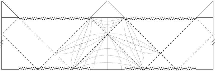
Figure 2 The lines in this diagram illustrate constant ˜ η and ˜ χ surfaces.
Figure 2 The lines in this diagram illustrate constant ˜ η and ˜ χ surfaces.CC-BY · From the PDF
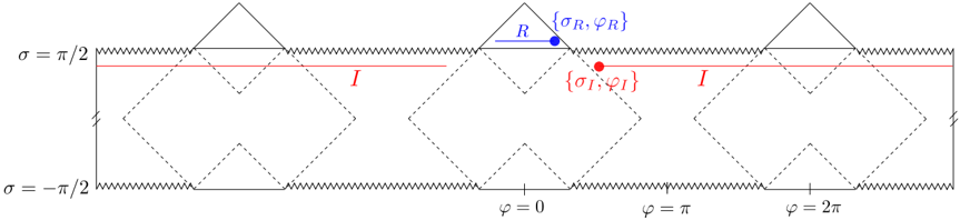
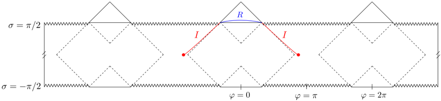
Figure 3 Island region I for entropy of region R in an n = 3 universe. The entropy on the complement of R ∪ I factorizes into the sum of the entropies on the two intervals; the endpoints of one of the two intervals are given by { σ I , ϕ I } and { σ R , ϕ R } as appears in (3.1).
Figure 3 Island region I for entropy of region R in an n = 3 universe. The entropy on the complement of R ∪ I factorizes into the sum of the entropies on the two intervals; the endpoints of one of the two intervals are given by { σ I , ϕ I } and { σ R , ϕ R } as appears in (3.1).CC-BY · From the PDF
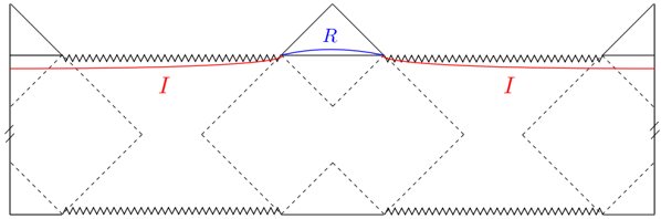
Figure 4 The 'purity' saddle which gives S = 0 for the entropy of one of the two hats in an n = 2 universe.
Figure 4 The 'purity' saddle which gives S = 0 for the entropy of one of the two hats in an n = 2 universe.CC-BY · From the PDF
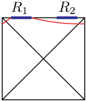
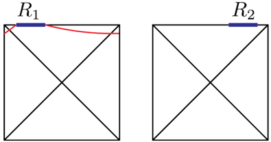
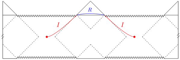
Figure 5 We imagine taking global de Sitter and freezing two regions near I + pictured in red. We integrate over the geometry away from these intervals. Naively, there is a puzzle since the entanglement wedge for one of the intervals appears to encompass the whole universe, since the spatial cross sections are compact. The naive entanglement wedge for R 2 is pictured in blue.
Figure 5 We imagine taking global de Sitter and freezing two regions near I + pictured in red. We integrate over the geometry away from these intervals. Naively, there is a puzzle since the entanglement wedge for one of the intervals appears to encompass the whole universe, since the spatial cross sections are compact. The naive entanglement wedge for R 2 is pictured in blue.CC-BY · From the PDF
Figure 6 The true saddle for the problem of two regions near I + is actually two disconnected universes, with each region in its own copy of the original spacetime.
Figure 6 The true saddle for the problem of two regions near I + is actually two disconnected universes, with each region in its own copy of the original spacetime.CC-BY · From the PDF
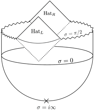
Figure 7 The connected, two-hat saddle which we are interested in studying. Here we have illustrated the Lorentzian to Euclidean continuation of this saddle from the σ = 0 line. This is a hemisphere of curvature R = 2 but with a conical excess at σ = i ∞ , the south pole of the hemisphere. The conical singularity has an opening angle of 4 πn . For n hats, it would have an opening angle of 2 πn .
Figure 7 The connected, two-hat saddle which we are interested in studying. Here we have illustrated the Lorentzian to Euclidean continuation of this saddle from the σ = 0 line. This is a hemisphere of curvature R = 2 but with a conical excess at σ = i ∞ , the south pole of the hemisphere. The conical singularity has an opening angle of 4 πn . For n hats, it would have an opening angle of 2 πn .CC-BY · From the PDF
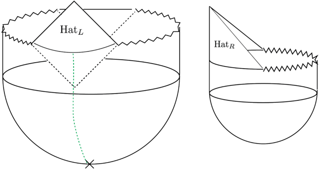
Figure 8 If we insert a conical singularity at a position which references only one of the hats, instead of both simultaneously, the dominant saddle will be two disconnected universes illustrated here. If we define the conical singularity with respect to the Hat L , then Hat L will be in a universe with angle 4 π and another, fluctuating asymptotically inflating region. Hat R will be off in its own 2 π universe. We have schematically illustrated the procedure of tying the conical singularity to a hat by the green dashed line. To prevent the saddle illustrated here from dominating the path integral, we need to tie the position of the conical singularity to both hats simultaneously. We discuss some ways of doing this in the main text.
Figure 8 If we insert a conical singularity at a position which references only one of the hats, instead of both simultaneously, the dominant saddle will be two disconnected universes illustrated here. If we define the conical singularity with respect to the Hat L , then Hat L will be in a universe with angle 4 π and another, fluctuating asymptotically inflating region. Hat R will be off in its own 2 π universe. We have schematically illustrated the procedure of tying the conical singularity to a hat by the green dashed line. To prevent the saddle illustrated here from dominating the path integral, we need to tie the position of the conical singularity to both hats simultaneously. We discuss some ways of doing this in the main text.CC-BY · From the PDF
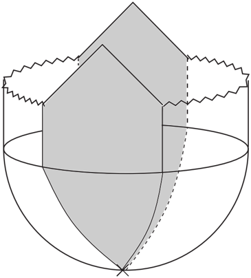
Figure 9 One could make the two-hat connected saddle dominate the path integral by freezing some portion of the geometry in the interior. A natural choice is to freeze all regions with some dilaton value φ ≥ 0 . Here we show the saddle where we have frozen everything filled in with gray. Note that when we include c/ ˜ φ r corrections to this solution then the frozen region actually includes a neighborhood of the conical singularity.
Figure 9 One could make the two-hat connected saddle dominate the path integral by freezing some portion of the geometry in the interior. A natural choice is to freeze all regions with some dilaton value φ ≥ 0 . Here we show the saddle where we have frozen everything filled in with gray. Note that when we include c/ ˜ φ r corrections to this solution then the frozen region actually includes a neighborhood of the conical singularity.CC-BY · From the PDF
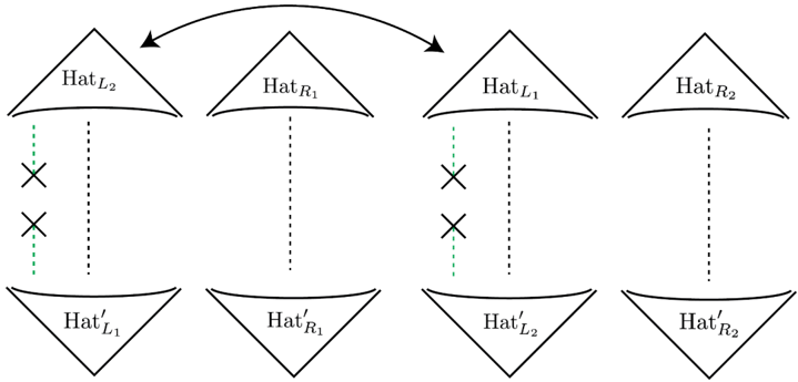
Figure 10 This figure illustrates what happens if the frozen portion of the geometry is only connected to one hat, in this case Hat L . The green-dashed lines schematically represent the frozen portion of the geometry. In this case, Hat L from replica 1 can be swapped with Hat L from replica 2 and so the dominant saddle will just be two copies of the saddle which dominates the norm, 〈 HH f | HH f 〉 . In other words, Tr [ ρ 2 ] = 〈 HH f | HH f 〉 2 where ρ is the unnormalized density matrix. The double-headed arrow indicates that the left hats from each replica have been swapped.
Figure 10 This figure illustrates what happens if the frozen portion of the geometry is only connected to one hat, in this case Hat L . The green-dashed lines schematically represent the frozen portion of the geometry. In this case, Hat L from replica 1 can be swapped with Hat L from replica 2 and so the dominant saddle will just be two copies of the saddle which dominates the norm, 〈 HH f | HH f 〉 . In other words, Tr [ ρ 2 ] = 〈 HH f | HH f 〉 2 where ρ is the unnormalized density matrix. The double-headed arrow indicates that the left hats from each replica have been swapped.CC-BY · From the PDF
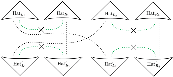
Figure 11 We illustrate the boundary conditions associated to computing the purity, Tr [ ρ 2 L ] , for the state on Hat L in the Hartle-Hawking state with modified boundary conditions, where the conical singularity (marked by 'X') is inserted in the frozen portion of the geometry. The prime denotes bra vs. ket and the subscript denotes replica number. Since this dressing ties hats of the same replica number to each other, we see that the quantum extremal surface (or its Renyi-2 analog), which gave an answer of S 2 = 0 for each hat, is excluded. The only possibility is the analog of the 'Hawking' saddle, which gives a non-zero answer for S 2 .
Figure 11 We illustrate the boundary conditions associated to computing the purity, Tr [ ρ 2 L ] , for the state on Hat L in the Hartle-Hawking state with modified boundary conditions, where the conical singularity (marked by 'X') is inserted in the frozen portion of the geometry. The prime denotes bra vs. ket and the subscript denotes replica number. Since this dressing ties hats of the same replica number to each other, we see that the quantum extremal surface (or its Renyi-2 analog), which gave an answer of S 2 = 0 for each hat, is excluded. The only possibility is the analog of the 'Hawking' saddle, which gives a non-zero answer for S 2 .CC-BY · From the PDF
Figure 12 The impure saddle for region R with n = 2 .
Figure 12 The impure saddle for region R with n = 2 .CC-BY · From the PDF
Figure 13 The impure saddle for region R with n = 3 .
Figure 13 The impure saddle for region R with n = 3 .CC-BY · From the PDF
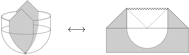
Figure 14 On the left we have reproduced figure 9, corresponding to the Euclidean preparation of a 4 π universe with frozen regions denoted in gray. On the right we have the Euclidean preparation of the thermofield double in AdS coupled to frozen flat-space 'wing' regions. The solid black line in the middle is the time-reflection symmetric point where the Euclidean manifold is pasted to the Lorentzian manifold. These two situations are analogous.
Figure 14 On the left we have reproduced figure 9, corresponding to the Euclidean preparation of a 4 π universe with frozen regions denoted in gray. On the right we have the Euclidean preparation of the thermofield double in AdS coupled to frozen flat-space 'wing' regions. The solid black line in the middle is the time-reflection symmetric point where the Euclidean manifold is pasted to the Lorentzian manifold. These two situations are analogous.CC-BY · From the PDF
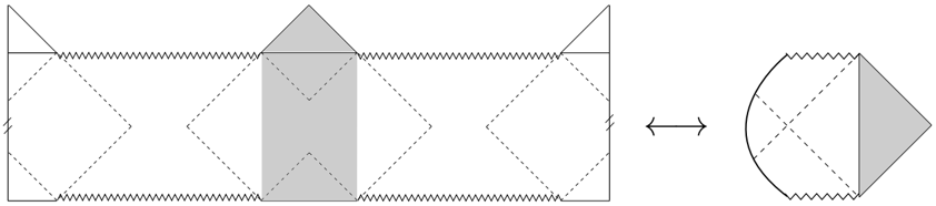
Figure 15 On the right we have a pure-state black hole with an end-of-the-world brane behind the horizon. This means that the single wing system (plus boundary) encodes the entire bulk, and has fine-grained entropy S = 0 . This corresponds to unfreezing one of the two frozen regions in the TFD in figure 14. It is analogous to a single frozen hat region in dS, shown on the left. In this case the theory in the hat has fine-grained entropy S = 0 and encodes the entire universe on its own.
Figure 15 On the right we have a pure-state black hole with an end-of-the-world brane behind the horizon. This means that the single wing system (plus boundary) encodes the entire bulk, and has fine-grained entropy S = 0 . This corresponds to unfreezing one of the two frozen regions in the TFD in figure 14. It is analogous to a single frozen hat region in dS, shown on the left. In this case the theory in the hat has fine-grained entropy S = 0 and encodes the entire universe on its own.CC-BY · From the PDF
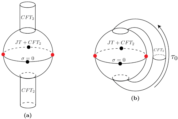
Figure 16 In the figure on the left, we imagine attaching two semi-infinite cylinders to holes at the north and south poles of the sphere. Here we have exaggerated the size of the holes relative to the size of the sphere. This prepares the CFT matter state in the vacuum on the circle, as was considered in section 2. On the right, we imagine making the CFT state thermal. This will raise the energy in the spacetime and make the wormholes longer upon analytic continuation. The red dots denote points of maximal dilaton and the black dots denote points of minimal dilaton along the σ = 0 time slice.
Figure 16 In the figure on the left, we imagine attaching two semi-infinite cylinders to holes at the north and south poles of the sphere. Here we have exaggerated the size of the holes relative to the size of the sphere. This prepares the CFT matter state in the vacuum on the circle, as was considered in section 2. On the right, we imagine making the CFT state thermal. This will raise the energy in the spacetime and make the wormholes longer upon analytic continuation. The red dots denote points of maximal dilaton and the black dots denote points of minimal dilaton along the σ = 0 time slice.CC-BY · From the PDF
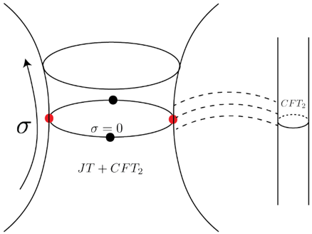
Figure 17 Here we illustrate the Lorentzian interpretations of the Euclidean saddles shown in figure 16. The idea is that for finite τ 0 these saddles describe a situation where a closed dS 2 universe with multiple inflating and crunching regions is encoded in a CFT 2 on a spatial circle. The dashed lines signify the thermal entanglement between the closed universe and the CFT.
Figure 17 Here we illustrate the Lorentzian interpretations of the Euclidean saddles shown in figure 16. The idea is that for finite τ 0 these saddles describe a situation where a closed dS 2 universe with multiple inflating and crunching regions is encoded in a CFT 2 on a spatial circle. The dashed lines signify the thermal entanglement between the closed universe and the CFT.CC-BY · From the PDF

Verification

Claims the paper makes

The claims and statistics of this paper haven’t been checked yet.

Run the check — free, no account needed. It reads the open-access text and checks the sources it cites.

A few free checks a day · papers already verified open instantly · results are public

Claims other papers make about this one

Each is checked against this paper’s own text: does it say what the citing paper says it does?

Self-check

Percentages, sums and reported differences re-computed from the paper’s own numbers.

The self-check needs the paper’s full text.

Citations

Cites

Research works printed but not linked: 35

  1. G.W. Gibbons and S.W. Hawking, Action Integrals and Partition Functions in Quantum Gravity, Phys. Rev. D 15 (1977) 2752 [INSPIRE]. · DOI · Paper page
  2. B. Freivogel, Y. Sekino, L. Susskind and C.-P. Yeh, A Holographic framework for eternal inflation, Phys. Rev. D 74 (2006) 086003 [hep-th/0606204] [INSPIRE]. · DOI · Paper page
  3. Y. Chen, V. Gorbenko and J. Maldacena, Bra-ket wormholes in gravitationally prepared states, JHEP 02 (2021) 009 [arXiv:2007.16091] [INSPIRE]. · DOI
  4. T. Hartman, Y. Jiang and E. Shaghoulian, Islands in cosmology, JHEP 11 (2020) 111 [arXiv:2008.01022] [INSPIRE]. · DOI
  5. J.M. Maldacena, Non-Gaussian features of primordial fluctuations in single field inflationary models, JHEP 05 (2003) 013 [astro-ph/0210603] [INSPIRE]. · DOI · Paper page
  6. A. Strominger, The dS / CFT correspondence, JHEP 10 (2001) 034 [hep-th/0106113] [INSPIRE]. · DOI
  7. R. Bousso, The Holographic principle for general backgrounds, Class. Quant. Grav. 17 (2000) 997 [hep-th/9911002] [INSPIRE]. · DOI
  8. R. Bousso, Positive vacuum energy and the N bound, JHEP 11 (2000) 038 [hep-th/0010252] [INSPIRE]. · DOI · Paper page
  9. T. Banks and W. Fischler, M theory observables for cosmological space-times, RUNHETC-2001-5 (2001), hep-th/0102077 [INSPIRE]. · arXiv
  10. T. Banks, W. Fischler and S. Paban, Recurrent nightmares? Measurement theory in de Sitter space, JHEP 12 (2002) 062 [hep-th/0210160] [INSPIRE]. · DOI
  11. T. Banks and W. Fischler, An Upper bound on the number of e-foldings, UTTG-04-03 (2003), astro-ph/0307459 [INSPIRE]. · arXiv
  12. T. Banks, B. Fiol and A. Morisse, Towards a quantum theory of de Sitter space, JHEP 12 (2006) 004 [hep-th/0609062] [INSPIRE]. · DOI
  13. T. Banks and W. Fischler, Holographic Inflation Revised, in S. Saunders, J. Silk, J.D. Barrow and K. Chamcham eds., The Philosophy of Cosmology, part III (2017) pp. 241–262 [arXiv:1501.01686] [INSPIRE]. · DOI
  14. T. Banks and W. Fischler, The holographic spacetime model of cosmology, Int. J. Mod. Phys. D 27 (2018) 1846005 [arXiv:1806.01749] [INSPIRE]. · DOI
  15. T. Banks and W. Fischler, Holographic Space-time, Newton‘s Law, and the Dynamics of Horizons, arXiv:2003.03637 [INSPIRE]. · arXiv
  16. L. Susskind, Three Impossible Theories, arXiv:2107.11688 [INSPIRE]. · arXiv
  17. E. Shaghoulian, The central dogma and cosmological horizons, JHEP 01 (2022) 132 [arXiv:2110.13210] [INSPIRE]. · DOI
  18. D. Anninos, G.S. Ng and A. Strominger, Future Boundary Conditions in De Sitter Space, JHEP 02 (2012) 032 [arXiv:1106.1175] [INSPIRE]. · DOI
  19. S.E. Aguilar-Gutierrez, A. Chatwin-Davies, T. Hertog, N. Pinzani-Fokeeva and B. Robinson, Islands in Multiverse Models, JHEP 11 (2021) 212 [arXiv:2108.01278] [INSPIRE]. · DOI
  20. B.S. Kay and R.M. Wald, Theorems on the Uniqueness and Thermal Properties of Stationary, Nonsingular, Quasifree States on Space-Times with a Bifurcate Killing Horizon, Phys. Rept. 207 (1991) 49 [INSPIRE]. · DOI · Paper page
  21. S. Gao and R.M. Wald, Theorems on gravitational time delay and related issues, Class. Quant. Grav. 17 (2000) 4999 [gr-qc/0007021] [INSPIRE]. · DOI
  22. F. Leblond, D. Marolf and R.C. Myers, Tall tales from de Sitter space 1: Renormalization group flows, JHEP 06 (2002) 052 [hep-th/0202094] [INSPIRE]. · DOI
  23. D. Harlow, The Ryu–Takayanagi Formula from Quantum Error Correction, Commun. Math. Phys. 354 (2017) 865 [arXiv:1607.03901] [INSPIRE]. · DOI
  24. D. Harlow and J.-q. Wu, Algebra of diffeomorphism-invariant observables in Jackiw-Teitelboim gravity, JHEP 05 (2022) 097 [arXiv:2108.04841] [INSPIRE]. · DOI
  25. C. Akers and P. Rath, Holographic Renyi Entropy from Quantum Error Correction, JHEP 05 (2019) 052 [arXiv:1811.05171] [INSPIRE]. · DOI · Paper page
  26. J. Feldbrugge, J.-L. Lehners and N. Turok, Lorentzian Quantum Cosmology, Phys. Rev. D 95 (2017) 103508 [arXiv:1703.02076] [INSPIRE]. · DOI · Paper page
  27. J. Hartle, S.W. Hawking and T. Hertog, Local Observation in Eternal inflation, Phys. Rev. Lett. 106 (2011) 141302 [arXiv:1009.2525] [INSPIRE]. · DOI
  28. J. Hartle and T. Hertog, One Bubble to Rule Them All, Phys. Rev. D 95 (2017) 123502 [arXiv:1604.03580] [INSPIRE]. · DOI
  29. V. Balasubramanian, A. Kar and T. Ugajin, Islands in de Sitter space, JHEP 02 (2021) 072 [arXiv:2008.05275] [INSPIRE]. · DOI
  30. E. Shaghoulian and L. Susskind, Entanglement in De Sitter space, JHEP 08 (2022) 198 [arXiv:2201.03603] [INSPIRE]. · DOI
  31. S. Cooper, M. Rozali, B. Swingle, M. Van Raamsdonk, C. Waddell and D. Wakeham, Black hole microstate cosmology, JHEP 07 (2019) 065 [arXiv:1810.10601] [INSPIRE]. · DOI
  32. M. Van Raamsdonk, Cosmology from confinement?, JHEP 03 (2022) 039 [arXiv:2102.05057] [INSPIRE]. · DOI
  33. S. Antonini, P. Simidzija, B. Swingle and M. Van Raamsdonk, Cosmology from the vacuum, arXiv:2203.11220 [INSPIRE]. · arXiv
  34. B. Freivogel, V.E. Hubeny, A. Maloney, R.C. Myers, M. Rangamani and S. Shenker, Inflation in AdS/CFT, JHEP 03 (2006) 007 [hep-th/0510046] [INSPIRE]. · DOI
  35. A. Belin, J. de Boer, J. Kruthoff, B. Michel, E. Shaghoulian and M. Shyani, Universality of sparse d > 2 conformal field theory at large N, JHEP 03 (2017) 067 [arXiv:1610.06186] [INSPIRE]. · DOI · Paper page

Cited by

See all 22

Metadata

Authors
Levine, A., & Shaghoulian, E.
Venue
Journal of High Energy Physics
Published
2023-02-17
Volume
2023
Issue
2
ISSN
1029-8479
Cited by
22
References
8
Language
en

About these checks

Registry, retraction, Cites and statistics results are computed, not judged, with one exception: a printed reference that no index lists is read once by a model before it counts as a citation error. Claims are extracted by a model and kept only when their quote appears verbatim in the text; each cited source is then checked, with a model’s help, for whether it says what the claim relies on. Those verdicts can be wrong — read the claim’s quote and the cited source before relying on one.

Statistics and arithmetic are recomputed, not judged.

Confidence bands are shown only for fields calibrated on our annotated test set. None is calibrated yet, so no band is shown.

What counts as a claim ›How we measure confidence ›How we check this ›

Are you an author, or do you see a problem with this page? Request a review

Data sources

Bibliographic data: Semantic Scholar, OpenAlex, Crossref.

Contains information from the Semantic Scholar Academic Graph Datasets, made available under the ODC Attribution License (ODC-BY 1.0).

Semantic Scholar’s data is described in: Kinney, R., et al. (2023). The Semantic Scholar Open Data Platform. arXiv:2301.10140.