Neutralizing topological obstructions to bubbles of nothing

TL;DR

The paper gives bottom-up constructions of bubble-of-nothing decays that are topologically obstructed by flux, Wilson lines, or incompatible fermion spin structures, showing how dynamical membranes or gauge fields can neutralize the obstruction. It finds new branch structure and a lower bound on brane tension in flux-stabilized models, and identifies Euclidean Reissner-Nordström as the relevant instanton for Wilson-line/fermion obstructions.

Key findings

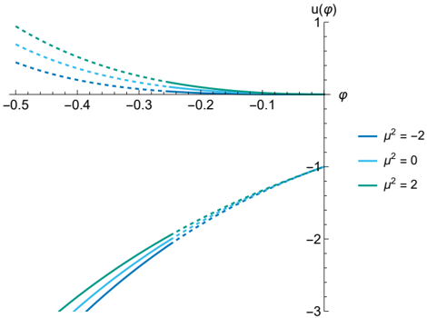
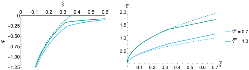
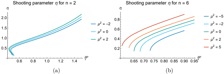
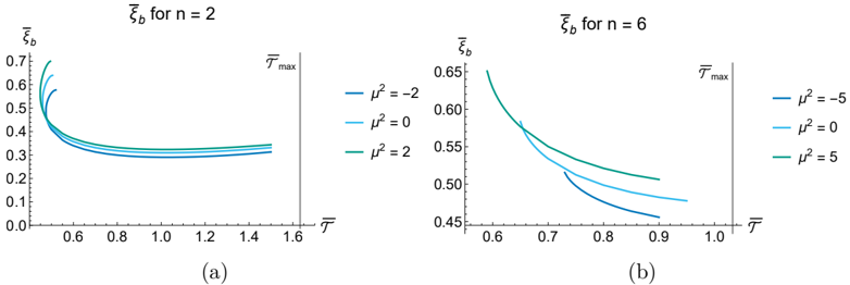
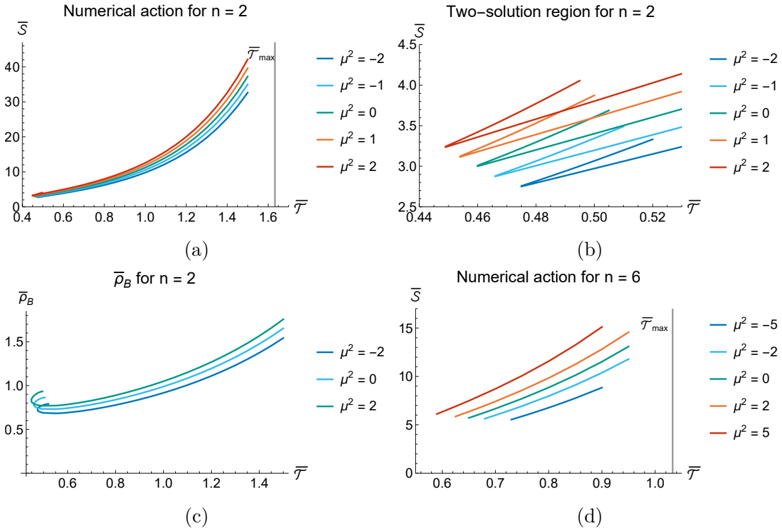
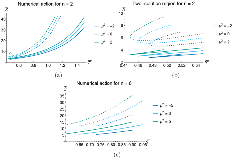
• For flux-stabilized internal spheres, BON decay requires co-nucleation with a charged membrane; the authors find two branches of solutions that merge at a minimal superextremal tension \(T_{\min}\), below which no viable solutions were found.
• The on-shell action grows faster than linearly with brane tension \(T\). For \(n=2\), \(\mu=0\), they report \(S(T=0.5)\approx 3\) and \(S(T=1.25)\approx 52\), and universe-lifetime bounds \(|Q|\gtrsim 20 g_0\) at \(T\simeq0.5\) and \(|Q|\gtrsim 10 g_0\) at \(T\simeq1.25\); for \(n=6\), \(|Q|\gtrsim150 g_0\) at \(T\simeq0.65\) and \(|Q|\gtrsim96 g_0\) at \(T\simeq0.95\).
• For Wilson operators and incompatible fermions, the relevant bubble is the Euclidean Reissner-Nordström black hole, and the ordinary decay exponent is modified by \(1/g^2\) effects; the Euclidean action is \(S_E \approx \frac{\pi^2 R_0^2}{\kappa_4}+\frac{2\pi^2 A_{5,0}^2}{g_4^2}\) for \(1/g_4^2\ll R_0^2/\kappa_4\).
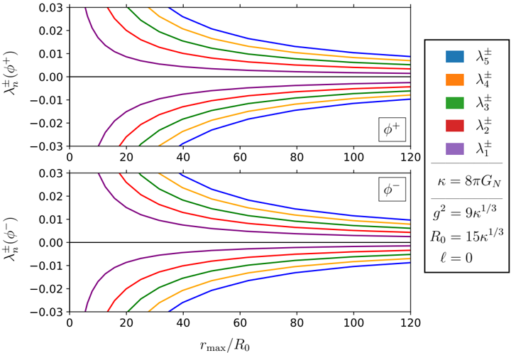
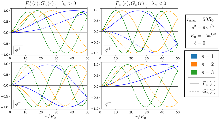
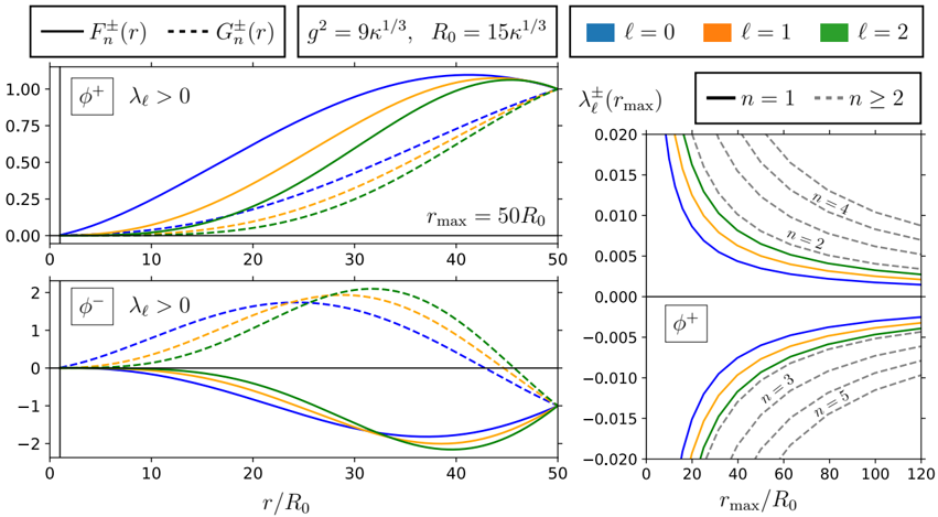
• A numerical Dirac spectrum on this background shows no isolated zero mode; eigenvalues converge to zero like \(1/r_{\max}\) as the cutoff grows. The mechanism can operate in softly broken gauged 5D supergravity, but the paper says only in rather exotic circumstances.

Methods

• Flux case: dimensionally reduce \(4+n\)-dimensional Einstein gravity with an \(n\)-sphere, flux, and a thin charged brane; formulate a Coleman-De Luccia problem with nonstandard boundary conditions, derive jump conditions, and solve numerically by shooting for \(n=2\) and \(n=6\) with potentials including \(\mu^2\).
• Wilson/fermion case: study 5D Kaluza-Klein theory with a background Wilson line or massive fermions, make the gauge field dynamical, and use the Euclidean Reissner-Nordström solution to Einstein-Maxwell equations.
• Dirac spectrum: solve the Dirac equation on the Euclidean Reissner-Nordström background numerically, using conformal transformation to a product manifold and point-and-shoot with Dirichlet boundary conditions.

Limitations

• The paper states that the flux analysis uses a thin-brane, full-screening approximation where all flux is screened inside the brane radius, treating the brane as smeared rather than localized; it says a more physically accurate treatment could alter the properties found.
• The paper states numerical difficulties: the upper branch for \(n=2\) is only found for restricted \(T\), the shooting method becomes unreliable near \(T_{\min}\) and \(T_{\max}\), and for \(n=6\) no second solution branch was found before numerical precision limits.
• The paper states that in the Wilson-line section it ignores the stabilizing radial modulus and the holonomy potential \(V(A_5)\), assuming a relevant minimum away from the origin; it also notes the Dirac spectrum discussion is “somewhat tangential.”