Student or educator? Sign up with your school email and get 6 months of Pro free.
Cited by 15

The DOI matches its Crossref record; 3 of the 3 references it cites were found in a registry or an index.

Bubble of nothing decays of unstable theories

Draper, Patrick, Garcia, Isabel Garcia, Lillard, Benjamin·2021·Physical Review D

Overview

The claims and statistics of this paper haven’t been checked yet.

Run the check — free, no account needed. It reads the open-access text and checks the sources it cites.

A few free checks a day · papers already verified open instantly · results are public

Integrity signals

Registry

Crossref · 10.1103/physrevd.104.l121701

Cites

3 of 3 references verified0 citation errors · 0 not checkable

Statistics

Figures

Image 1
CC-BY · From the PDF
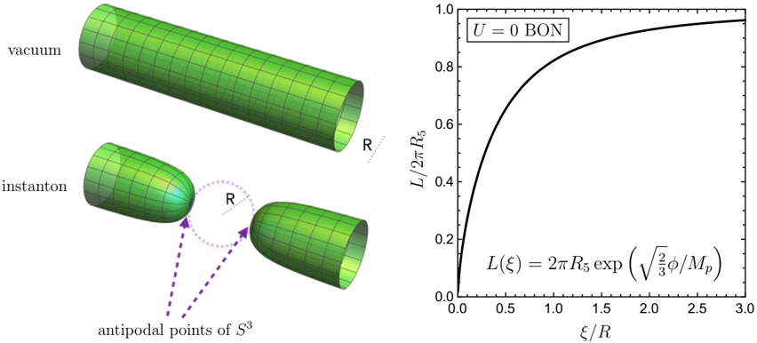
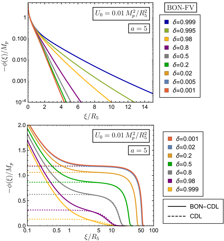
Figure 3 Diagram R5 Figure 11: Just L (   ) 5 Figure 2 . Left: diagram showing the geometry of the KK false vacuum ('vacuum') and BON ('instanton') solutions. The r direction lies along the symmetry axis, with the periodic y coordinate along the azimuth. In the false vacuum, φ ≡ 0 , and the KK radius is independent of r . For Witten's bubble, the KK radius approaches zero near r ≳ R 5 , whereas far away from the bubble wall the geometry asymptotically approaches that of the false vacuum. Right: after dimensional reduction, the scalar modulus φ describes the proper length of the KK circle, L . As a function of the CDL coordinate, defined in eq. (2.20), L vanishes at ξ = 0 , corresponding to the location of bubble wall, whereas L ≃ 2 πR 5 in the asymptotic region ξ ≫ R 5 .
Figure 3 Diagram R5 Figure 11: Just L ( ) 5 Figure 2 . Left: diagram showing the geometry of the KK false vacuum ('vacuum') and BON ('instanton') solutions. The r direction lies along the symmetry axis, with the periodic y coordinate along the azimuth. In the false vacuum, φ ≡ 0 , and the KK radius is independent of r . For Witten's bubble, the KK radius approaches zero near r ≳ R 5 , whereas far away from the bubble wall the geometry asymptotically approaches that of the false vacuum. Right: after dimensional reduction, the scalar modulus φ describes the proper length of the KK circle, L . As a function of the CDL coordinate, defined in eq. (2.20), L vanishes at ξ = 0 , corresponding to the location of bubble wall, whereas L ≃ 2 πR 5 in the asymptotic region ξ ≫ R 5 .CC-BY · From the PDF
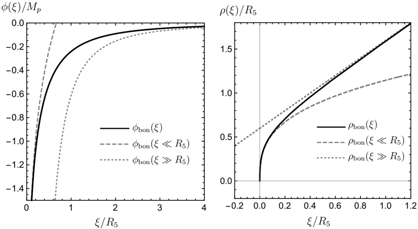
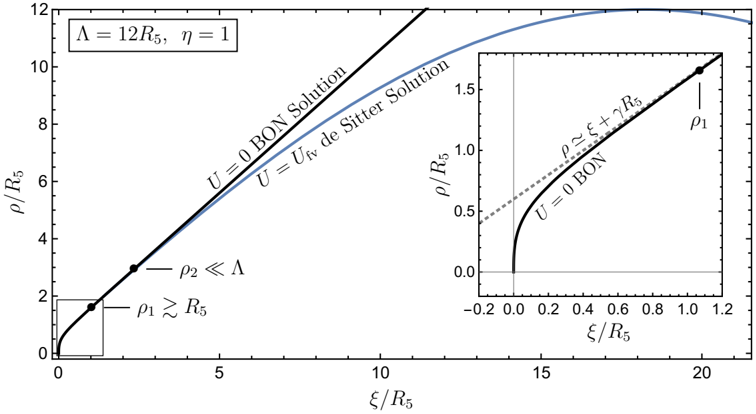
Figure 6 Cartoon 3 Figure 3 . The five-dimensional Euclidean Schwarzschild gravitational instanton, or Witten's BON, expressed in terms of the degrees of freedom φ bon ( ξ ) ( left ) and ρ bon ( ξ ) ( right ) of the corresponding CDL problem. The behavior of the solutions in the near-horizon ( ξ ≪ R 5 ) and asymptotic ( ξ ≫ R 5 ) regimes is indicated in the figure, following eq. (2.21) and eq. (2.22), respectively.
Figure 6 Cartoon 3 Figure 3 . The five-dimensional Euclidean Schwarzschild gravitational instanton, or Witten's BON, expressed in terms of the degrees of freedom φ bon ( ξ ) ( left ) and ρ bon ( ξ ) ( right ) of the corresponding CDL problem. The behavior of the solutions in the near-horizon ( ξ ≪ R 5 ) and asymptotic ( ξ ≫ R 5 ) regimes is indicated in the figure, following eq. (2.21) and eq. (2.22), respectively.CC-BY · From the PDF
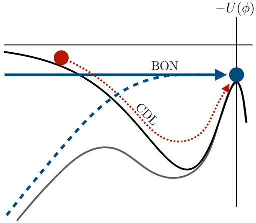
Figure 6 Cartoon 3 Figure 4 . A diagram comparing the BON and CDL boundary conditions. The BON initial conditions φ (0) → -∞ , φ ′ → + ∞ ensure that φ ( ξ ) quickly approaches the false vacuum. Its approach to φ ( ξ ) → φ fv is determined by the details of the potential, which is approximately quadratic in the neighborhood of φ ≈ φ fv . This direct approach to φ fv is indicated by the straight blue line in the figure. The CDL solution, on the other hand, begins at finite φ (0) = φ CDL with φ ′ (0) = 0 . It subsequently 'rolls' in the inverted potential, as indicated by the dashed red line, until it approaches φ fv . In the dashed blue line we show a second BON example, one in which the potential U ( φ → -∞ ) diverges (with -U ( φ ) shown in dark gray). The φ ′ (0) → ∞ BON initial conditions can compensate for the divergence in U ( φ ) , so that there is a BON solution even if there is no corresponding CDL solution for that potential.
Figure 6 Cartoon 3 Figure 4 . A diagram comparing the BON and CDL boundary conditions. The BON initial conditions φ (0) → -∞ , φ ′ → + ∞ ensure that φ ( ξ ) quickly approaches the false vacuum. Its approach to φ ( ξ ) → φ fv is determined by the details of the potential, which is approximately quadratic in the neighborhood of φ ≈ φ fv . This direct approach to φ fv is indicated by the straight blue line in the figure. The CDL solution, on the other hand, begins at finite φ (0) = φ CDL with φ ′ (0) = 0 . It subsequently 'rolls' in the inverted potential, as indicated by the dashed red line, until it approaches φ fv . In the dashed blue line we show a second BON example, one in which the potential U ( φ → -∞ ) diverges (with -U ( φ ) shown in dark gray). The φ ′ (0) → ∞ BON initial conditions can compensate for the divergence in U ( φ ) , so that there is a BON solution even if there is no corresponding CDL solution for that potential.CC-BY · From the PDF
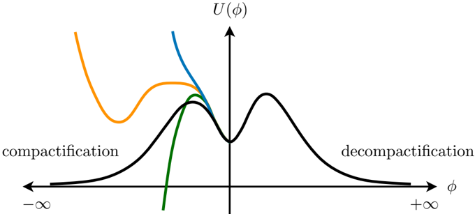
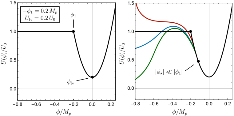
antipodal points of S 3 Figure 4: Diagram R5 2 1.5 Figure 9: Piecewise toy potential U (   ), together with more realistic examples 4 Figure 5 . Left: the piecewise potential U toy ( φ ) from eq. (3.17), with φ 1 = -0 . 2 M p and U fv = 0 . 2 U 0 . Right: the quantity φ ⋆ = -m 2 R 2 5 2 √ 3 2 M p indicates the point where the potential U ( φ ) begins to have a noticeable effect on the equation of motion for φ (see the discussion around eq. (3.45)). For φ ≪ φ ⋆ , φ ( ξ ) is well approximated by the Witten BON solution, even if the potential U ( φ ) is large. This feature greatly enhances the utility of the piecewise quadratic toy model. All three of the 'realistic' smooth potentials will have similar solutions for φ ( ξ ) and ρ ( ξ ) , despite the significant differences in their asymptotic φ →-∞ limits, as long as mR 5 ≪ 1 is small enough that U ( | φ | ≤ | φ ⋆ | ) remains approximately quadratic.
antipodal points of S 3 Figure 4: Diagram R5 2 1.5 Figure 9: Piecewise toy potential U ( ), together with more realistic examples 4 Figure 5 . Left: the piecewise potential U toy ( φ ) from eq. (3.17), with φ 1 = -0 . 2 M p and U fv = 0 . 2 U 0 . Right: the quantity φ ⋆ = -m 2 R 2 5 2 √ 3 2 M p indicates the point where the potential U ( φ ) begins to have a noticeable effect on the equation of motion for φ (see the discussion around eq. (3.45)). For φ ≪ φ ⋆ , φ ( ξ ) is well approximated by the Witten BON solution, even if the potential U ( φ ) is large. This feature greatly enhances the utility of the piecewise quadratic toy model. All three of the 'realistic' smooth potentials will have similar solutions for φ ( ξ ) and ρ ( ξ ) , despite the significant differences in their asymptotic φ →-∞ limits, as long as mR 5 ≪ 1 is small enough that U ( | φ | ≤ | φ ⋆ | ) remains approximately quadratic.CC-BY · From the PDF
Image 6
CC-BY · From the PDF
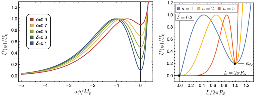
Figure 20 Potential U (   ) Figure 7 . Left: the scalar potential ˆ U ( φ ) , as given in eq. (4.1), for several values of δ ≡ U fv /U 0 , as indicated in the figure. A potential of this kind, exhibiting a de Sitter vacuum that is separated by a finite barrier from the compactification limit, admits hybrid BON-CDL and BON-HM instanton solutions. Right: to illustrate the physical meaning of a , we show ˆ U with fixed δ = 0 . 2 as a function of the proper length of the KK direction, L = 2 πR 5 exp (√ 2 3 φ/M p ) . Larger values of a create a steeper potential near the false vacuum at L = 2 πR 5 , while also flattening U ( L ) at L ≪ πR 5 .
Figure 20 Potential U ( ) Figure 7 . Left: the scalar potential ˆ U ( φ ) , as given in eq. (4.1), for several values of δ ≡ U fv /U 0 , as indicated in the figure. A potential of this kind, exhibiting a de Sitter vacuum that is separated by a finite barrier from the compactification limit, admits hybrid BON-CDL and BON-HM instanton solutions. Right: to illustrate the physical meaning of a , we show ˆ U with fixed δ = 0 . 2 as a function of the proper length of the KK direction, L = 2 πR 5 exp (√ 2 3 φ/M p ) . Larger values of a create a steeper potential near the false vacuum at L = 2 πR 5 , while also flattening U ( L ) at L ≪ πR 5 .CC-BY · From the PDF
Image 8
CC-BY · From the PDF
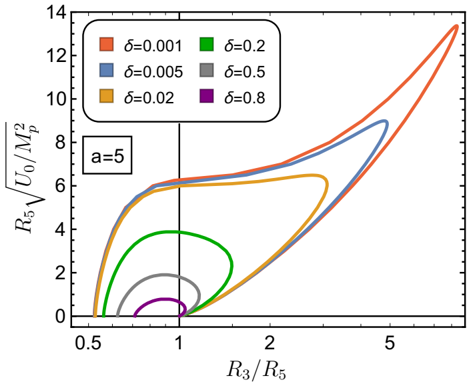
Figure 14 Parameter space R 3 /R 5 Figure 9 . The trajectories of the BON bounce solutions in the ( η, R 5 ) plane are shown for a = 5 and various 0 < δ < 1 . Each value of δ has a BON-FV branch of solutions, with R 3 ≈ R 5 ( φ 0 ≈ 0 ) in the u 0 ≪ 1 limit where the potential becomes unimportant. The BON-CDL branch of solutions has R 3 < R 5 ( φ 0 ≈ φ cdl ) in the u 0 ≪ 1 limit, and an action ∆ S ≈ S CDL that is large compared to π 2 M 2 p R 2 5 . When u 0 ≳ 1 , the potential U ( φ ) is no longer a small perturbation to the Witten bubble, and we find that the BON-FV and BON-CDL branches merge together, with u 0 for the bounce solution bounded from above by some u max 0 . For u 0 > u max 0 , all solutions to the equations of motion are of the overshoot type. As δ → 0 the CDL action diverges as δ -1 , and the unification of the BON-FV and BON-CDL branches is pushed to ever-larger values of u 0 ≫ 1 .
Figure 14 Parameter space R 3 /R 5 Figure 9 . The trajectories of the BON bounce solutions in the ( η, R 5 ) plane are shown for a = 5 and various 0 < δ < 1 . Each value of δ has a BON-FV branch of solutions, with R 3 ≈ R 5 ( φ 0 ≈ 0 ) in the u 0 ≪ 1 limit where the potential becomes unimportant. The BON-CDL branch of solutions has R 3 < R 5 ( φ 0 ≈ φ cdl ) in the u 0 ≪ 1 limit, and an action ∆ S ≈ S CDL that is large compared to π 2 M 2 p R 2 5 . When u 0 ≳ 1 , the potential U ( φ ) is no longer a small perturbation to the Witten bubble, and we find that the BON-FV and BON-CDL branches merge together, with u 0 for the bounce solution bounded from above by some u max 0 . For u 0 > u max 0 , all solutions to the equations of motion are of the overshoot type. As δ → 0 the CDL action diverges as δ -1 , and the unification of the BON-FV and BON-CDL branches is pushed to ever-larger values of u 0 ≫ 1 .CC-BY · From the PDF
Image 10
CC-BY · From the PDF
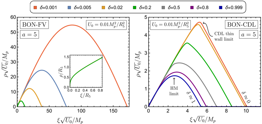
Figure 31 ⇢ ( ⇠ ) with inset Left: BON-FV Right: BON-CdL 15 Figure 11 . Profiles for ρ ( ξ ) for U 0 R 2 5 /M 2 p = 0 . 01 on the BON-FV ( left ) and BON-CDL ( right ) branches. For the BON-FV branch the solutions for ρ ( ξ ) are nearly identical to the false vacuum solution ρ fv ( ξ ) for ξ ≳ R 5 . This encompasses the majority of the domain 0 ≤ ξ ≤ ξ max ≈ π Λ , which is why we only show δ = 0 . 001 . . . 0 . 2 . For the BON-CDL solutions, the profiles for ρ ( ξ ) follow the ξ ≫ R 5 linear growth of eq. (2.22) out to ξ ≳ 10 R 5 or larger, with a relatively sharp transition from ρ ′ ≈ 1 to ρ ′ ≈ -1 in the case of small δ . As δ → 1 , the BON-CDL solutions for ρ ( ξ ) more closely match the Hawking-Moss behavior ρ ( ξ ) ≈ ρ HM ( ξ ) for all ξ ≳ R 5 , even though the a = 5 CDL and HM solutions for φ ( ξ ) are distinct.
Figure 31 ⇢ ( ⇠ ) with inset Left: BON-FV Right: BON-CdL 15 Figure 11 . Profiles for ρ ( ξ ) for U 0 R 2 5 /M 2 p = 0 . 01 on the BON-FV ( left ) and BON-CDL ( right ) branches. For the BON-FV branch the solutions for ρ ( ξ ) are nearly identical to the false vacuum solution ρ fv ( ξ ) for ξ ≳ R 5 . This encompasses the majority of the domain 0 ≤ ξ ≤ ξ max ≈ π Λ , which is why we only show δ = 0 . 001 . . . 0 . 2 . For the BON-CDL solutions, the profiles for ρ ( ξ ) follow the ξ ≫ R 5 linear growth of eq. (2.22) out to ξ ≳ 10 R 5 or larger, with a relatively sharp transition from ρ ′ ≈ 1 to ρ ′ ≈ -1 in the case of small δ . As δ → 1 , the BON-CDL solutions for ρ ( ξ ) more closely match the Hawking-Moss behavior ρ ( ξ ) ≈ ρ HM ( ξ ) for all ξ ≳ R 5 , even though the a = 5 CDL and HM solutions for φ ( ξ ) are distinct.CC-BY · From the PDF
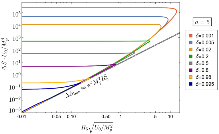
Figure 24 Action as function of R 5 Figure 12 . The de Sitter-subtracted Euclidean action ∆ S is shown in units of M 4 p /U 0 as a function of R 5 , for a = 5 and various 0 < δ < 1 . The dashed gray line shows the ∆ S ≈ π 2 M 2 p R 2 5 expectation from the small u 0 ≪ 1 limit of the BON-FV solutions. It tracks the numericallycomputed action closely on this branch for all u 0 ≪ 1 . This branch is always of lowest action and determines the tunneling rate. On the BON-CDL branch the action approaches a constant, the ordinary CDL action ∆ S ≈ S CDL , which is large compared to M 4 p /U 0 for δ ≲ 0 . 5 . For δ ≪ 1 , S CDL ≈ 24 π 2 M 4 p / ( δ · U 0 ) , grows as 1 /δ . At larger values of u 0 , where π 2 M 2 p R 2 5 ∼ ∆ S CDL , the BON-FV and BON-CDL branches of bounce solutions meet. (This method of estimating the value of u 0 = U 0 R 2 5 /M 2 p at which the two branches meet becomes imprecise once u 0 ≳ 1 , where π 2 M 2 p R 5 is no longer a good approximation to the BON-FV action.)
Figure 24 Action as function of R 5 Figure 12 . The de Sitter-subtracted Euclidean action ∆ S is shown in units of M 4 p /U 0 as a function of R 5 , for a = 5 and various 0 < δ < 1 . The dashed gray line shows the ∆ S ≈ π 2 M 2 p R 2 5 expectation from the small u 0 ≪ 1 limit of the BON-FV solutions. It tracks the numericallycomputed action closely on this branch for all u 0 ≪ 1 . This branch is always of lowest action and determines the tunneling rate. On the BON-CDL branch the action approaches a constant, the ordinary CDL action ∆ S ≈ S CDL , which is large compared to M 4 p /U 0 for δ ≲ 0 . 5 . For δ ≪ 1 , S CDL ≈ 24 π 2 M 4 p / ( δ · U 0 ) , grows as 1 /δ . At larger values of u 0 , where π 2 M 2 p R 2 5 ∼ ∆ S CDL , the BON-FV and BON-CDL branches of bounce solutions meet. (This method of estimating the value of u 0 = U 0 R 2 5 /M 2 p at which the two branches meet becomes imprecise once u 0 ≳ 1 , where π 2 M 2 p R 5 is no longer a good approximation to the BON-FV action.)CC-BY · From the PDF
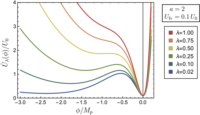
Figure 16 Potential U (   , ⇤ ) Figure 13 . The scalar potential ˆ U λ ( φ ) of eq. (5.4), for several values of λ ≡ Λ CC 5 M 2 p /U 0 .
Figure 16 Potential U ( , ⇤ ) Figure 13 . The scalar potential ˆ U λ ( φ ) of eq. (5.4), for several values of λ ≡ Λ CC 5 M 2 p /U 0 .CC-BY · From the PDF
Image 14
CC-BY · From the PDF
Image 15
CC-BY · From the PDF
Image 16
CC-BY · From the PDF

Verification

Claims the paper makes

The claims and statistics of this paper haven’t been checked yet.

Run the check — free, no account needed. It reads the open-access text and checks the sources it cites.

A few free checks a day · papers already verified open instantly · results are public

Claims other papers make about this one

Each is checked against this paper’s own text: does it say what the citing paper says it does?

Self-check

Percentages, sums and reported differences re-computed from the paper’s own numbers.

The self-check needs the paper’s full text.

Citations

Cites

Show all 3 references

Research works printed but not linked: 50

  1. 10.1086/307221 · DOI · Paper page
  2. 10.1111/j.1365-2966.2009.15812.x · DOI · Paper page
  3. 10.1051/0004-6361/201833910 · DOI · Paper page
  4. 10.1142/S0217751X01003937 · DOI · Paper page
  5. P. K. Townsend, 2003, Proceedings of the 14th International Congress on Mathematical Physics, Lisbon, Portugal
  6. 10.1088/1126-6708/2007/12/095 · DOI · Paper page
  7. 10.1002/prop.201000053 · DOI
  8. 10.1007/JHEP09(2011)052 · DOI
  9. 10.1007/JHEP02(2015)146 · DOI
  10. 10.1103/PhysRevLett.115.071305 · DOI
  11. 10.1007/JHEP03(2017)102 · DOI
  12. 10.1007/JHEP03(2018)083 · DOI
  13. 10.1103/PhysRevD.97.046010 · DOI
  14. 10.1007/JHEP10(2018)022 · DOI
  15. 10.1142/S0218271818300070 · DOI
  16. 10.1007/JHEP04(2019)008 · DOI
  17. 10.1007/JHEP06(2019)019 · DOI
  18. 10.1007/JHEP08(2019)141 · DOI
  19. 10.1002/prop.202000089 · DOI
  20. 10.1103/PhysRevD.68.046005 · DOI
  21. 10.1088/1126-6708/2005/03/007 · DOI · Paper page
  22. 10.1007/JHEP11(2019)075 · DOI
  23. 10.1016/j.physletb.2018.11.018 · DOI
  24. 10.1103/PhysRevD.68.026006 · DOI · Paper page
  25. 10.1103/PhysRevD.70.046005 · DOI · Paper page
  26. 10.1103/PhysRevD.15.2929 · DOI · Paper page
  27. 10.1103/PhysRevD.16.1248 · DOI · Paper page
  28. 10.1103/PhysRevD.16.1762 · DOI · Paper page
  29. 10.1016/0550-3213(82)90007-4 · DOI · Paper page
  30. 10.1016/S0550-3213(00)00255-8 · DOI · Paper page
  31. 10.1016/0370-2693(91)90618-Z · DOI · Paper page
  32. 10.1103/PhysRevD.66.026005 · DOI · Paper page
  33. 10.1007/JHEP08(2020)128 · DOI · Paper page
  34. 10.1103/PhysRevD.77.024004 · DOI
  35. 10.1088/1475-7516/2016/10/002 · DOI · Paper page
  36. 10.1007/JHEP12(2020)032 · DOI · Paper page
  37. 10.1103/PhysRevD.82.086015 · DOI
  38. 10.1088/1475-7516/2010/10/029 · DOI
  39. 10.1103/PhysRevD.84.043518 · DOI · Paper page
  40. 10.1103/PhysRevD.96.026016 · DOI · Paper page
  41. 10.1088/1126-6708/2004/09/037 · DOI
  42. 10.1016/S0550-3213(99)00037-1 · DOI
  43. 10.1103/PhysRevD.60.095008 · DOI
  44. 10.1016/S0370-2693(98)00979-4 · DOI
  45. 10.1103/PhysRevD.66.095003 · DOI
  46. 10.1016/S0550-3213(03)00573-X · DOI
  47. 10.1103/PhysRevLett.113.111802 · DOI
  48. 10.1007/JHEP12(2015)005 · DOI
  49. 10.1103/PhysRevD.91.126014 · DOI
  50. 10.1103/PhysRevD.97.126017 · DOI

Cited by

See all 15

Metadata

Authors
Draper, P., Garcia, I. G., & Lillard, B.
Venue
Physical Review D
Published
2021-12-02
Volume
104
Issue
12
ISSN
  • 2470-0010
  • 2470-0029
Cited by
15
References
3
Language
en
Funders
  • U.S. Department of Energy (DE-SC0015655)
  • Gordon and Betty Moore Foundation (GBMF7392)
  • National Science Foundation (PHY-1748958)

About these checks

Registry, retraction, Cites and statistics results are computed, not judged, with one exception: a printed reference that no index lists is read once by a model before it counts as a citation error. Claims are extracted by a model and kept only when their quote appears verbatim in the text; each cited source is then checked, with a model’s help, for whether it says what the claim relies on. Those verdicts can be wrong — read the claim’s quote and the cited source before relying on one.

Statistics and arithmetic are recomputed, not judged.

Confidence bands are shown only for fields calibrated on our annotated test set. None is calibrated yet, so no band is shown.

What counts as a claim ›How we measure confidence ›How we check this ›

Are you an author, or do you see a problem with this page? Request a review

How to cite

Cite CoChat for the checks on this page, and the paper for its own findings.

This page
CoChat. (2026). Citation check: Bubble of nothing decays of unstable theories. https://app.cochat.ai/papers/10.1103/physrevd.104.l121701
The paper
Draper, P., Garcia, I. G., & Lillard, B. (2021). Bubble of nothing decays of unstable theories. Physical Review D. https://doi.org/10.1103/physrevd.104.l121701

Data sources

Bibliographic data: Semantic Scholar, OpenAlex, Crossref.

Contains information from the Semantic Scholar Academic Graph Datasets, made available under the ODC Attribution License (ODC-BY 1.0).

Semantic Scholar’s data is described in: Kinney, R., et al. (2023). The Semantic Scholar Open Data Platform. arXiv:2301.10140.