

The DOI matches its Crossref record; 9 of the 9 references it cites were found in a registry or an index.
De Sitter decays to infinity
Abstract
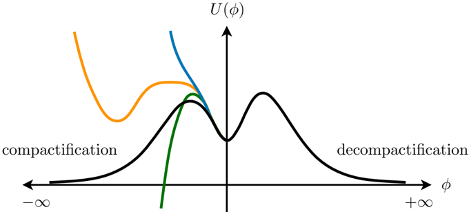
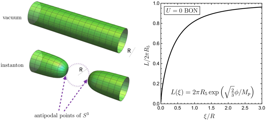
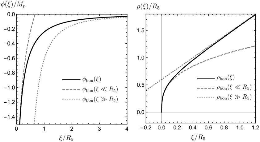
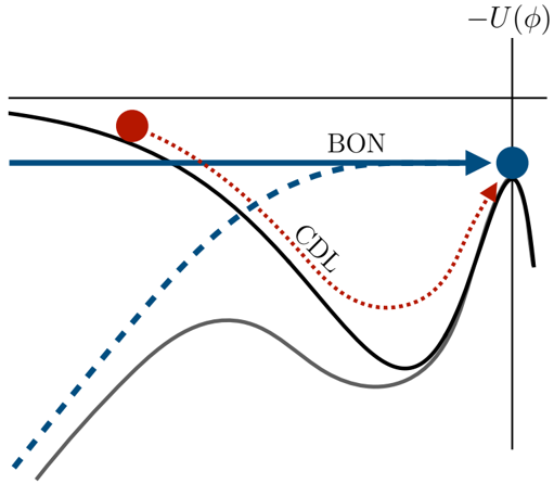
Bubbles of nothing are a class of vacuum decay processes present in some theories with compactified extra dimensions. We investigate the existence and properties of bubbles of nothing in models where the scalar pseudomoduli controlling the size of the extra dimensions are stabilized at positive vacuum energy, which is a necessary feature of any realistic model. We map the construction of bubbles of nothing to a four-dimensional Coleman-De Luccia problem and establish necessary conditions on the asymptotic behavior of the scalar potential for the existence of suitable solutions. We perform detailed analyses in the context of five-dimensional theories with metastable dS 4× S1 vacua, using analytic approximations and numerical methods to calculate the decay rate. We find that bubbles of nothing sometimes exist in potentials with no ordinary Coleman-De Luccia decay process, and that in the examples we study, when both processes exist, the bubble of nothing decay rate is typically faster. Our methods can be generalized to other stabilizing potentials and internal manifolds.
Overview
The claims and statistics of this paper haven’t been checked yet.
Run the check — free, no account needed. It reads the open-access text and checks the sources it cites.
Integrity signals
Registry
Cites
Statistics
Figures
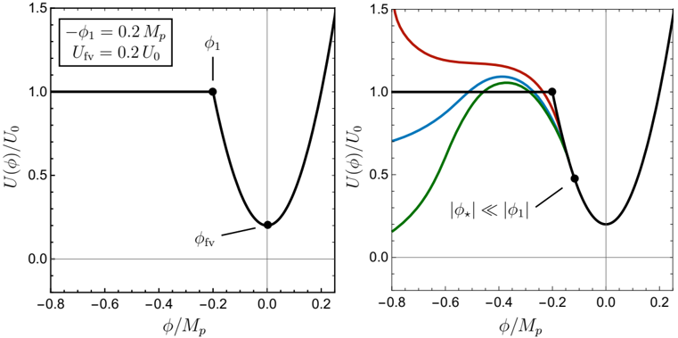
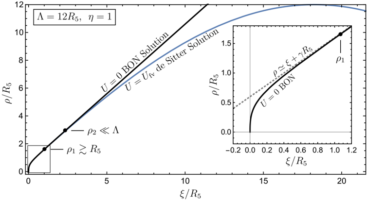
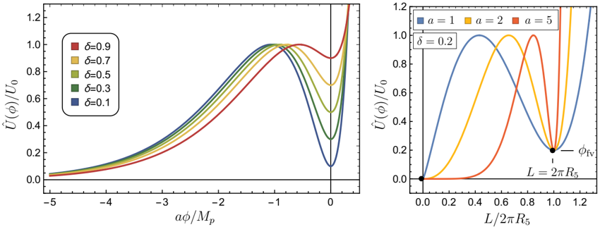
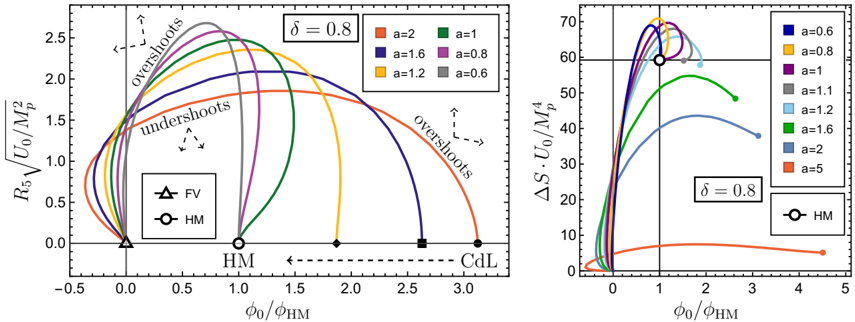
Verification
Claims the paper makes
The claims and statistics of this paper haven’t been checked yet.
Run the check — free, no account needed. It reads the open-access text and checks the sources it cites.
Claims other papers make about this one
Each is checked against this paper’s own text: does it say what the citing paper says it does?
In the citing paper
“The CDL equations have no smooth solution in the bubble-of-nothing class in the presence of this term [16,17].”
From Neutralizing topological obstructions to bubbles of nothing (2023) · cites this paper as [17]
Self-check
Percentages, sums and reported differences re-computed from the paper’s own numbers.
The self-check needs the paper’s full text.
Citations
Cites
Gravitational effects on and of vacuum decay
Coleman, S., & De Luccia, F. (1980) · Physical Review D · doi:10.1103/physrevd.21.3305 · Cited by 1,537 · cited 5×
“where σ is the bubble wall tension given by σ ' ∫ φfv φtv dφ √ 2(U(φ)− U(φfv)) [29].”
BackgroundMethodInfluentialSupercooled phase transitions in the very early universe
Hawking, S. W., & Moss, I. L. (1982) · Physics Letters B · doi:10.1016/0370-2693(82)90946-7 · Cited by 816
Instability of the Kaluza-Klein vacuum
Witten, E. (1982) · Nuclear Physics B · doi:10.1016/0550-3213(82)90007-4 · Cited by 595
Could the universe have recovered from a slow first-order phase transition?
Guth, A. H., & Weinberg, E. J. (1983) · Nuclear Physics B · doi:10.1016/0550-3213(83)90307-3 · Cited by 576
Is the superstring weakly coupled?
Dine, M., & Seiberg, N. (1985) · Physics Letters B · doi:10.1016/0370-2693(85)90927-x · Cited by 392
Nothing is certain in string compactifications
Etxebarria, I. G., Montero, M., Sousa, K., & Valenzuela, I. (2020) · Journal of High Energy Physics · doi:10.1007/jhep12(2020)032 · Cited by 87
Spontaneous decompactification
Giddings, S. B., & Myers, R. C. (2004) · Physical Review D · doi:10.1103/physrevd.70.046005 · Cited by 59
Dibitetto, G., Petri, N., & Schillo, M. (2020) · Journal of High Energy Physics · doi:10.1007/jhep08(2020)040 · Cited by 45
Bubbles of nothing and supersymmetric compactifications
Blanco-Pillado, J. J., Shlaer, B., Sousa, K., & Urrestilla, J. (2016) · Journal of Cosmology and Astroparticle Physics · doi:10.1088/1475-7516/2016/10/002 · Cited by 27
Research works printed but not linked: 47
- Supernova Cosmology Project collaboration, Measurements of Ω and Λ from 42 high redshift supernovae, Astrophys. J. 517 (1999) 565 [astro-ph/9812133] [INSPIRE]. · arXiv
- SDSS collaboration, Baryon acoustic oscillations in the Sloan Digital Sky Survey data release 7 galaxy sample, Mon. Not. Roy. Astron. Soc. 401 (2010) 2148 [arXiv:0907.1660] [INSPIRE]. · arXiv
- Planck collaboration, Planck 2018 results. VI. Cosmological parameters, Astron. Astrophys. 641 (2020) A6 [Erratum ibid. 652 (2021) C4] [arXiv:1807.06209] [INSPIRE]. · arXiv
- S. Kachru, R. Kallosh, A. D. Linde and S. P. Trivedi, De Sitter vacua in string theory, Phys. Rev. D 68 (2003) 046005 [hep-th/0301240] [INSPIRE]. · DOI
- V. Balasubramanian, P. Berglund, J. P. Conlon and F. Quevedo, Systematics of moduli stabilisation in Calabi-Yau flux compactifications, JHEP 03 (2005) 007 [hep-th/0502058] [INSPIRE]. · DOI · Paper page
- J. M. Maldacena and C. Núñez, Supergravity description of field theories on curved manifolds and a no go theorem, Int. J. Mod. Phys. A 16 (2001) 822 [hep-th/0007018] [INSPIRE]. · DOI · Paper page
- P. K. Townsend, Cosmic acceleration and M-theory, in 14th International congress on mathematical physics, (2003), pg. 655 [hep-th/0308149] [INSPIRE]. · arXiv
- M. P. Hertzberg, S. Kachru, W. Taylor and M. Tegmark, Inflationary constraints on type IIA string theory, JHEP 12 (2007) 095 [arXiv:0711.2512] [INSPIRE]. · DOI · Paper page
- T. Wrase and M. Zagermann, On classical de Sitter vacua in string theory, Fortsch. Phys. 58 (2010) 906 [arXiv:1003.0029] [INSPIRE]. · DOI
- G. Shiu and Y. Sumitomo, Stability constraints on classical de Sitter vacua, JHEP 09 (2011) 052 [arXiv:1107.2925] [INSPIRE]. · DOI
- I. Bena, M. Graña, S. Kuperstein and S. Massai, Giant tachyons in the landscape, JHEP 02 (2015) 146 [arXiv:1410.7776] [INSPIRE]. · DOI
- D. Kutasov, T. Maxfield, I. Melnikov and S. Sethi, Constraining de Sitter space in string theory, Phys. Rev. Lett. 115 (2015) 071305 [arXiv:1504.00056] [INSPIRE]. · DOI
- D. Andriot and J. Blåbäck, Refining the boundaries of the classical de Sitter landscape, JHEP 03 (2017) 102 [Erratum ibid. 03 (2018) 083] [arXiv:1609.00385] [INSPIRE]. · DOI
- J. Moritz, A. Retolaza and A. Westphal, Toward de Sitter space from ten dimensions, Phys. Rev. D 97 (2018) 046010 [arXiv:1707.08678] [INSPIRE]. · DOI
- S. Sethi, Supersymmetry breaking by fluxes, JHEP 10 (2018) 022 [arXiv:1709.03554] [INSPIRE]. · DOI
- U. H. Danielsson and T. Van Riet, What if string theory has no de Sitter vacua?, Int. J. Mod. Phys. D 27 (2018) 1830007 [arXiv:1804.01120] [INSPIRE]. · DOI
- Y. Hamada, A. Hebecker, G. Shiu and P. Soler, On brane gaugino condensates in 10d, JHEP 04 (2019) 008 [arXiv:1812.06097] [INSPIRE]. · DOI
- Y. Hamada, A. Hebecker, G. Shiu and P. Soler, Understanding KKLT from a 10d perspective, JHEP 06 (2019) 019 [arXiv:1902.01410] [INSPIRE]. · DOI
- F. Carta, J. Moritz and A. Westphal, Gaugino condensation and small uplifts in KKLT, JHEP 08 (2019) 141 [arXiv:1902.01412] [INSPIRE]. · DOI
- X. Gao, A. Hebecker and D. Junghans, Control issues of KKLT, Fortsch. Phys. 68 (2020) 2000089 [arXiv:2009.03914] [INSPIRE]. · DOI
- I. Basile and S. Lanza, De Sitter in non-supersymmetric string theories: no-go theorems and brane-worlds, JHEP 10 (2020) 108 [arXiv:2007.13757] [INSPIRE]. · DOI
- G. Obied, H. Ooguri, L. Spodyneiko and C. Vafa, De Sitter space and the swampland, arXiv:1806.08362 [INSPIRE]. · arXiv
- S. K. Garg and C. Krishnan, Bounds on slow roll and the de Sitter swampland, JHEP 11 (2019) 075 [arXiv:1807.05193] [INSPIRE]. · DOI
- H. Ooguri, E. Palti, G. Shiu and C. Vafa, Distance and de Sitter conjectures on the swampland, Phys. Lett. B 788 (2019) 180 [arXiv:1810.05506] [INSPIRE]. · DOI
- A. Bedroya and C. Vafa, Trans-Planckian censorship and the swampland, JHEP 09 (2020) 123 [arXiv:1909.11063] [INSPIRE]. · DOI
- S. B. Giddings, The fate of four-dimensions, Phys. Rev. D 68 (2003) 026006 [hep-th/0303031] [INSPIRE]. · DOI · Paper page
- M. Dine, P. J. Fox and E. Gorbatov, Catastrophic decays of compactified space-times, JHEP 09 (2004) 037 [hep-th/0405190] [INSPIRE]. · DOI
- M. Fabinger and P. Hořava, Casimir effect between world branes in heterotic M-theory, Nucl. Phys. B 580 (2000) 243 [hep-th/0002073] [INSPIRE]. · DOI · Paper page
- D. Brill and G. T. Horowitz, Negative energy in string theory, Phys. Lett. B 262 (1991) 437 [INSPIRE]. · DOI · Paper page
- S. P. De Alwis and A. T. Flournoy, Closed string tachyons and semiclassical instabilities, Phys. Rev. D 66 (2002) 026005 [hep-th/0201185] [INSPIRE]. · DOI · Paper page
- B. S. Acharya, Supersymmetry, Ricci flat manifolds and the string landscape, JHEP 08 (2020) 128 [arXiv:1906.06886] [INSPIRE]. · DOI · Paper page
- G. T. Horowitz, J. Orgera and J. Polchinski, Nonperturbative instability of AdS5 × S5/Zk, Phys. Rev. D 77 (2008) 024004 [arXiv:0709.4262] [INSPIRE]. · DOI
- J. J. Blanco-Pillado and B. Shlaer, Bubbles of nothing in flux compactifications, Phys. Rev. D 82 (2010) 086015 [arXiv:1002.4408] [INSPIRE]. · DOI
- A. R. Brown and A. Dahlen, Bubbles of nothing and the fastest decay in the landscape, Phys. Rev. D 84 (2011) 043518 [arXiv:1010.5240] [INSPIRE]. · DOI · Paper page
- J. J. Blanco-Pillado, H. S. Ramadhan and B. Shlaer, Decay of flux vacua to nothing, JCAP 10 (2010) 029 [arXiv:1009.0753] [INSPIRE]. · DOI
- H. Ooguri and L. Spodyneiko, New Kaluza-Klein instantons and the decay of AdS vacua, Phys. Rev. D 96 (2017) 026016 [arXiv:1703.03105] [INSPIRE]. · DOI · Paper page
- P. Draper, I. G. Garcia and B. Lillard, Bubble of nothing decays of unstable theories, Phys. Rev. D 104 (2021) L121701 [arXiv:2105.08068] [INSPIRE]. · DOI · Paper page
- S. R. Coleman, The fate of the false vacuum. 1. Semiclassical theory, Phys. Rev. D 15 (1977) 2929 [Erratum ibid. 16 (1977) 1248] [INSPIRE]. · DOI · Paper page
- C. G. Callan, Jr. and S. R. Coleman, The fate of the false vacuum. 2. First quantum corrections, Phys. Rev. D 16 (1977) 1762 [INSPIRE]. · DOI · Paper page
- L. G. Jensen and P. J. Steinhardt, Bubble nucleation and the Coleman-Weinberg model, Nucl. Phys. B 237 (1984) 176 [INSPIRE]. · DOI
- L. G. Jensen and P. J. Steinhardt, Bubble nucleation for flat potential barriers, Nucl. Phys. B 317 (1989) 693 [INSPIRE]. · DOI
- J. C. Hackworth and E. J. Weinberg, Oscillating bounce solutions and vacuum tunneling in de Sitter spacetime, Phys. Rev. D 71 (2005) 044014 [hep-th/0410142] [INSPIRE]. · DOI
- P. Batra and M. Kleban, Transitions between de Sitter minima, Phys. Rev. D 76 (2007) 103510 [hep-th/0612083] [INSPIRE]. · DOI
- P. Draper and S. Farkas, Transplanckian censorship and the local swampland distance conjecture, JHEP 01 (2020) 133 [arXiv:1910.04804] [INSPIRE]. · DOI
- A. R. Brown and A. Dahlen, On ‘nothing’ as an infinitely negatively curved spacetime, Phys. Rev. D 85 (2012) 104026 [arXiv:1111.0301] [INSPIRE]. · DOI
- C. Angelantonj, M. Cardella and N. Irges, An alternative for moduli stabilisation, Phys. Lett. B 641 (2006) 474 [hep-th/0608022] [INSPIRE]. · DOI
- A. Rajantie and S. Stopyra, Standard Model vacuum decay in a de Sitter background, Phys. Rev. D 97 (2018) 025012 [arXiv:1707.09175] [INSPIRE]. · DOI
Cited by
Neutralizing topological obstructions to bubbles of nothing
Draper, P., Lillard, B., & Skye, C. (2023) · Journal of High Energy Physics · doi:10.1007/jhep10(2023)049 · Cited by 5
Self-citation
Metadata
- Authors
- Draper, P., Garcia, I. G., & Lillard, B.
- Venue
- Journal of High Energy Physics
- Published
- 2021-12-21
- Volume
- 2021
- Issue
- 12
- ISSN
- 1029-8479
- Cited by
- 14
- References
- 9
- Language
- en
About these checks
Registry, retraction, Cites and statistics results are computed, not judged, with one exception: a printed reference that no index lists is read once by a model before it counts as a citation error. Claims are extracted by a model and kept only when their quote appears verbatim in the text; each cited source is then checked, with a model’s help, for whether it says what the claim relies on. Those verdicts can be wrong — read the claim’s quote and the cited source before relying on one.
Statistics and arithmetic are recomputed, not judged.
Confidence bands are shown only for fields calibrated on our annotated test set. None is calibrated yet, so no band is shown.
What counts as a claim ›How we measure confidence ›How we check this ›
Are you an author, or do you see a problem with this page? Request a review
Data sources
Bibliographic data: Semantic Scholar, OpenAlex, Crossref.
Contains information from the Semantic Scholar Academic Graph Datasets, made available under the ODC Attribution License (ODC-BY 1.0).
Semantic Scholar’s data is described in: Kinney, R., et al. (2023). The Semantic Scholar Open Data Platform. arXiv:2301.10140.
