CoChat

Planning and navigation as active inference

Open access
Kaplan, Raphael, Friston, Karl J. · 2018 · Biological Cybernetics

Published version of a preprint

The DOI matches its Crossref record; 98 of the 98 references it cites were found in a registry or an index.

Abstract

This paper introduces an active inference formulation of planning and navigation. It illustrates how the exploitation-exploration dilemma is dissolved by acting to minimise uncertainty (i.e. expected surprise or free energy). We use simulations of a maze problem to illustrate how agents can solve quite complicated problems using context sensitive prior preferences to form subgoals. Our focus is on how epistemic behaviour-driven by novelty and the imperative to reduce uncertainty about the world-contextualises pragmatic or goal-directed behaviour. Using simulations, we illustrate the underlying process theory with synthetic behavioural and electrophysiological responses during exploration of a maze and subsequent navigation to a target location. An interesting phenomenon that emerged from the simulations was a putative distinction between 'place cells'-that fire when a subgoal is reached-and 'path cells'-that fire until a subgoal is reached.

Overview

The claims and statistics of this paper haven’t been checked yet.

Free: it reads the open-access text and checks the first 5 claims that cite a source we can check. Create a free account to check every claim.

A few free checks a day · papers already verified open instantly · results are public

Integrity signals

Registry

Crossref · 10.1007/s00422-018-0753-2

Cites

98 of 98 references verified0 citation errors · 0 not checkable

Statistics

Figures

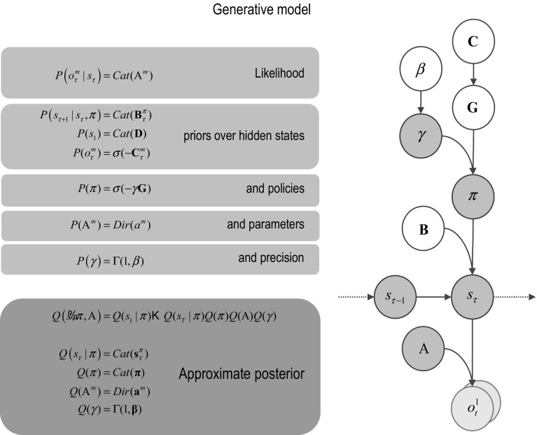
Fig. 1 Generative model and (approximate) posterior. A generative model specifies the joint probability of outcomes or consequences and their (latent or hidden) causes. Usually, the model is expressed in terms of a likelihood (the probability of consequences given causes) and priors over causes. When a prior depends upon a random variable, it is called an empirical prior. Here, the likelihood is specified by matrices A whose components are the probability of an outcome under each hidden state. The empirical priors in this instance pertain to transitions among hidden states B that depend upon action, where actions are determined probabilistically in terms of policies (sequences of actions denoted by π). The key aspect of this generative model is that policies are more probable a priori if they minimise the (path integral of) expected free energy G. Bayesian model inversion refers to the inverse mapping from consequences to causes, i.e. estimating the hidden states and other variables that cause outcomes. In variational Bayesian inversion, one has to specify the form of an approximate posterior distribution, which is provided in the lower panel. This particular form uses a mean field approximation, in which posterior beliefs are approximated by the product of marginal distributions over unknown quantities. Here, a mean field approximation is applied both posterior beliefs at different points in time, policies, parameters and precision. Cat and Dir referred to categorical and Dirichlet distributions, respectively. See the main text and Table 2 for a detailed explanation of the variables. The insert shows a graphical representation of the dependencies implied by the equations on the right
Fig. 1 Generative model and (approximate) posterior. A generative model specifies the joint probability of outcomes or consequences and their (latent or hidden) causes. Usually, the model is expressed in terms of a likelihood (the probability of consequences given causes) and priors over causes. When a prior depends upon a random variable, it is called an empirical prior. Here, the likelihood is specified by matrices A whose components are the probability of an outcome under each hidden state. The empirical priors in this instance pertain to transitions among hidden states B that depend upon action, where actions are determined probabilistically in terms of policies (sequences of actions denoted by π). The key aspect of this generative model is that policies are more probable a priori if they minimise the (path integral of) expected free energy G. Bayesian model inversion refers to the inverse mapping from consequences to causes, i.e. estimating the hidden states and other variables that cause outcomes. In variational Bayesian inversion, one has to specify the form of an approximate posterior distribution, which is provided in the lower panel. This particular form uses a mean field approximation, in which posterior beliefs are approximated by the product of marginal distributions over unknown quantities. Here, a mean field approximation is applied both posterior beliefs at different points in time, policies, parameters and precision. Cat and Dir referred to categorical and Dirichlet distributions, respectively. See the main text and Table 2 for a detailed explanation of the variables. The insert shows a graphical representation of the dependencies implied by the equations on the rightCC BY · PubMed Central
Fig. 2 Schematic overview of belief updating: the left panel lists the belief updates mediating perception, policy selection, precision and learning, while the left panel assigns the updates to various brain areas. This attribution is purely schematic and serves to illustrate an implicit functional anatomy. Here, we have assigned observed outcomes to representations in the pontine–geniculate occipital system, with visual (what) modalities entering an extrastriate stream and proprioceptive (where) modalities originating from the lateral geniculate nucleus (LGN) via the superficial layers of the superior colliculus. Hidden states encoding location have been associated with the hippocampal formation and association (parietal) cortex. The evaluation of policies, in terms of their (expected) free energy, has been placed in the caudate. Expectations about policies—assigned to the putamen—are used to create Bayesian model averages of future outcomes (e.g. in the frontal or parietal cortex). In addition, expected policies specify the most likely action (e.g. via the deep layers of the superior colliculus). Finally, the precision of beliefs about—confidence in—policies rests on updates to expected precision that have been assigned to the central tegmental area or substantia nigra (VTA/SN). The arrows denote message passing among the sufficient statistics of each marginal as might be mediated by extrinsic connections in the brain. The red arrow indicates activity-dependent plasticity. Please see appendix and Table 2 for an explanation of the equations and variables
Fig. 2 Schematic overview of belief updating: the left panel lists the belief updates mediating perception, policy selection, precision and learning, while the left panel assigns the updates to various brain areas. This attribution is purely schematic and serves to illustrate an implicit functional anatomy. Here, we have assigned observed outcomes to representations in the pontine–geniculate occipital system, with visual (what) modalities entering an extrastriate stream and proprioceptive (where) modalities originating from the lateral geniculate nucleus (LGN) via the superficial layers of the superior colliculus. Hidden states encoding location have been associated with the hippocampal formation and association (parietal) cortex. The evaluation of policies, in terms of their (expected) free energy, has been placed in the caudate. Expectations about policies—assigned to the putamen—are used to create Bayesian model averages of future outcomes (e.g. in the frontal or parietal cortex). In addition, expected policies specify the most likely action (e.g. via the deep layers of the superior colliculus). Finally, the precision of beliefs about—confidence in—policies rests on updates to expected precision that have been assigned to the central tegmental area or substantia nigra (VTA/SN). The arrows denote message passing among the sufficient statistics of each marginal as might be mediated by extrinsic connections in the brain. The red arrow indicates activity-dependent plasticity. Please see appendix and Table 2 for an explanation of the equations and variablesCC BY · PubMed Central
Fig. 3 Explorative, epistemic behaviour. Left panel: This figure reports the results of epistemic exploration for 32 (two move) trials (e.g. 64 saccadic eye movements). The maze shown in terms of closed (black) and open (white) locations. The magenta dots and lines correspond to the chosen path, while the large red dot denotes the final location. The agent starts (in this maze) at the entrance on the lower left. The key thing to observe in these results is that the trajectory very seldom repeats or crosses itself. This affords a very efficient search of state space, resolving ignorance about the consequences of occupying a particular location (in terms of the first—what—outcome; black vs. white). Right panel: this figure reports the likelihood of observing an open state (white), from each location, according to the concentration parameters of the likelihood matrix that have been accumulated during exploration (for the first—what—outcome modality). At the end of search, the posterior expectations change from 50% (grey) to high or low (white or black) in, and only in, those locations that have been visited. The underlying concentration parameters effectively remember what has been learned or accumulated during exploration—and can be used for planning, given a particular task set (as illustrated in Fig. 5)
Fig. 3 Explorative, epistemic behaviour. Left panel: This figure reports the results of epistemic exploration for 32 (two move) trials (e.g. 64 saccadic eye movements). The maze shown in terms of closed (black) and open (white) locations. The magenta dots and lines correspond to the chosen path, while the large red dot denotes the final location. The agent starts (in this maze) at the entrance on the lower left. The key thing to observe in these results is that the trajectory very seldom repeats or crosses itself. This affords a very efficient search of state space, resolving ignorance about the consequences of occupying a particular location (in terms of the first—what—outcome; black vs. white). Right panel: this figure reports the likelihood of observing an open state (white), from each location, according to the concentration parameters of the likelihood matrix that have been accumulated during exploration (for the first—what—outcome modality). At the end of search, the posterior expectations change from 50% (grey) to high or low (white or black) in, and only in, those locations that have been visited. The underlying concentration parameters effectively remember what has been learned or accumulated during exploration—and can be used for planning, given a particular task set (as illustrated in Fig. 5)CC BY · PubMed Central
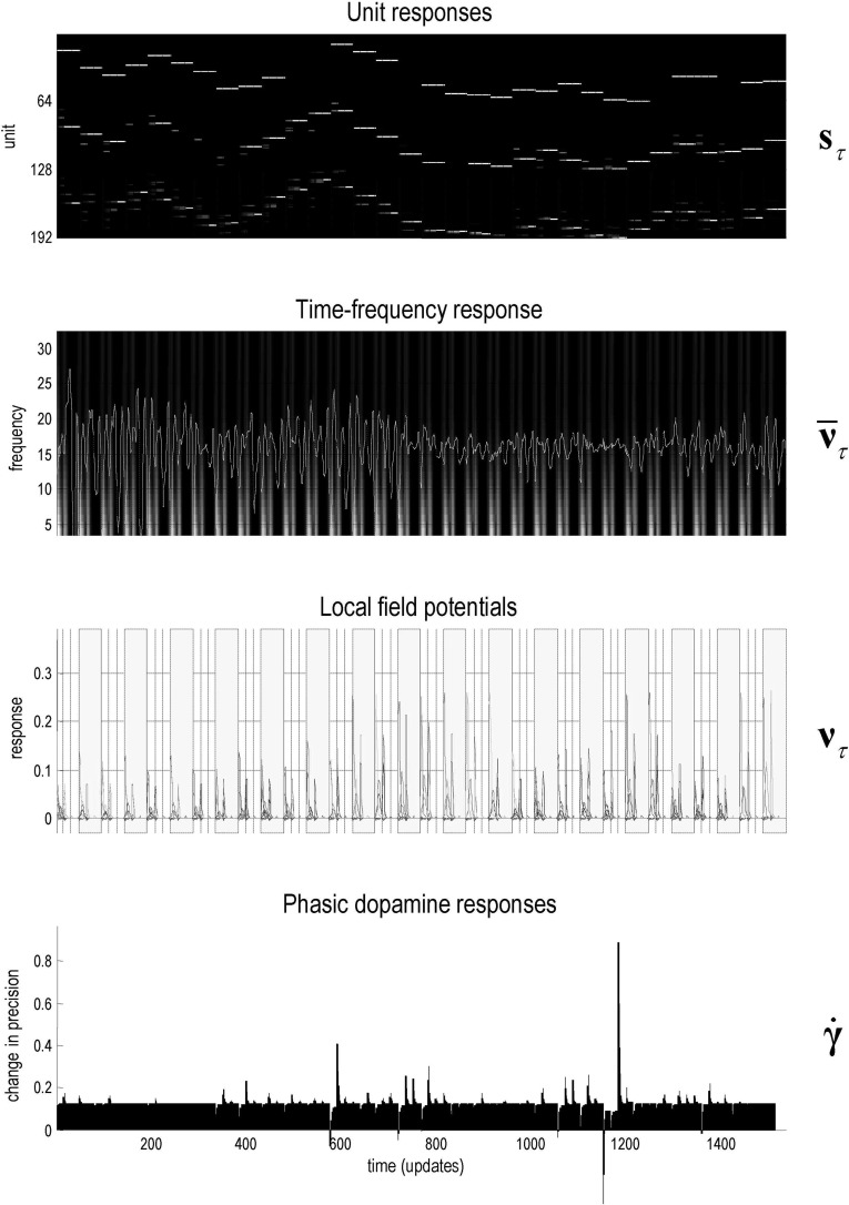
Fig. 4 Simulated electrophysiological responses during exploration: this figure reports the simulated electrophysiological responses during the epistemic search of the previous figure. Upper panel: this panel shows the activity (firing rate) of units encoding the expected location—over 32 trials—in image (raster) format. There are 192=64×3 units for each of the 64 locations over the three epochs between two saccades that constitute a trial. These responses are organised such that the upper rows encode the probability of alternative states in the first epoch, with subsequent epochs in lower rows. The simulated local field potentials for these units (i.e. log state prediction error) are shown in the middle panels. Second panel: this panel shows the response of the first hidden state unit (white line) after filtering at 4 Hz, superimposed upon a time–frequency decomposition of the local field potential (averaged over all units). The key observation here is that depolarisation in the 4 Hz range coincides with induced responses, including gamma activity. Third panel: these are the simulated local field potentials (i.e. depolarisation) for all (192) hidden state units (coloured lines). Note how visiting different locations evokes responses in distinct units of varying magnitude. Alternating trials (of two movements) are highlighted with grey bars. Lower panel: this panel illustrates simulated dopamine responses in terms of a mixture of precision and its rate of change (see Fig. 2). There phasic fluctuations reflect changes in precision or confidence based upon the mismatch between the free energy before and after observing outcomes (see Fig. 2) (colour figure online)
Fig. 4 Simulated electrophysiological responses during exploration: this figure reports the simulated electrophysiological responses during the epistemic search of the previous figure. Upper panel: this panel shows the activity (firing rate) of units encoding the expected location—over 32 trials—in image (raster) format. There are 192=64×3 units for each of the 64 locations over the three epochs between two saccades that constitute a trial. These responses are organised such that the upper rows encode the probability of alternative states in the first epoch, with subsequent epochs in lower rows. The simulated local field potentials for these units (i.e. log state prediction error) are shown in the middle panels. Second panel: this panel shows the response of the first hidden state unit (white line) after filtering at 4 Hz, superimposed upon a time–frequency decomposition of the local field potential (averaged over all units). The key observation here is that depolarisation in the 4 Hz range coincides with induced responses, including gamma activity. Third panel: these are the simulated local field potentials (i.e. depolarisation) for all (192) hidden state units (coloured lines). Note how visiting different locations evokes responses in distinct units of varying magnitude. Alternating trials (of two movements) are highlighted with grey bars. Lower panel: this panel illustrates simulated dopamine responses in terms of a mixture of precision and its rate of change (see Fig. 2). There phasic fluctuations reflect changes in precision or confidence based upon the mismatch between the free energy before and after observing outcomes (see Fig. 2) (colour figure online)CC BY · PubMed Central
Fig. 5 Planning and navigation: this figure shows the results of navigating to a target under a task set (i.e. prior preferences), after the maze has been learned (with concentration parameters of 128). These prior preferences render the closed (black) locations surprising and they are therefore avoided. Furthermore, the agent believes that it will move to locations that are successively closer to the target—as encoded by subgoals. Left panels: the upper panel shows the chosen trajectory that takes the shortest path to the target, using the same format as Fig. 3. The lower panel shows the final location and prior preferences in terms of prior probabilities. At this point, the start and end locations are identical—and the most attractive location is the target itself. As earlier points in navigation, the most attractive point is within the horizon of allowable policies. Middle panels: these show the prior preferences over eight successive trials (16 eye movements), using the same format as above. The preferred locations play the role of context sensitive subgoals, in the sense that subgoals lie within the horizon of the (short-term) policies entertained by the agent—and effectively act as a ‘carrot’ leading the agent to the target location. Right panel: these report the planning or goal-directed performance based upon partially observed mazes, using the simulations reported in Fig. 3. In other words, we assessed performance in terms of the number of moves before the target is acquired (latency) and the number of closed regions or disallowed locations visited en route (mistakes). These performance metrics were assessed during the accumulation of concentration parameters. This corresponds to the sort of performance one would expect to see when a subject was exposed to the maze for increasing durations (here, from one to 16 s of simulated time), before being asked to return to the start location and navigate to a target that is subsequently revealed
Fig. 5 Planning and navigation: this figure shows the results of navigating to a target under a task set (i.e. prior preferences), after the maze has been learned (with concentration parameters of 128). These prior preferences render the closed (black) locations surprising and they are therefore avoided. Furthermore, the agent believes that it will move to locations that are successively closer to the target—as encoded by subgoals. Left panels: the upper panel shows the chosen trajectory that takes the shortest path to the target, using the same format as Fig. 3. The lower panel shows the final location and prior preferences in terms of prior probabilities. At this point, the start and end locations are identical—and the most attractive location is the target itself. As earlier points in navigation, the most attractive point is within the horizon of allowable policies. Middle panels: these show the prior preferences over eight successive trials (16 eye movements), using the same format as above. The preferred locations play the role of context sensitive subgoals, in the sense that subgoals lie within the horizon of the (short-term) policies entertained by the agent—and effectively act as a ‘carrot’ leading the agent to the target location. Right panel: these report the planning or goal-directed performance based upon partially observed mazes, using the simulations reported in Fig. 3. In other words, we assessed performance in terms of the number of moves before the target is acquired (latency) and the number of closed regions or disallowed locations visited en route (mistakes). These performance metrics were assessed during the accumulation of concentration parameters. This corresponds to the sort of performance one would expect to see when a subject was exposed to the maze for increasing durations (here, from one to 16 s of simulated time), before being asked to return to the start location and navigate to a target that is subsequently revealedCC BY · PubMed Central
Fig. 6 Goal-directed exploration: this figure illustrates behavioural, mnemonic and electrophysiological responses over four searches, each comprising 8 trials (or 16 eye movements). Crucially, the agent started with a novel maze but was equipped with a task set in terms of prior preferences leading to the goal-directed navigation of the previous figure. Each row of panels corresponds to a successive search. Left panels: these report the path chosen (left) and posterior expectations of the likelihood mapping (right) as evidence is accumulated. However, here, the epistemic search is constrained by prior preferences that attract the target. This attraction is not complete and there are examples where epistemic value (i.e. novelty of a nearby location) overwhelms the pragmatic value of the target location—and the subject gives way to curiosity. However, having said that the subject never wanders far from the shortest path to the target, which she acquires optimally after the fourth attempt. Right panels: these show the corresponding evoked responses or simulated depolarisation in state units (upper panels) and the corresponding changes in expected precision that simulate dopaminergic responses (lower panels). The interesting observation here is the progressive attenuation of evoked responses in the state units as the subject becomes more familiar with the maze. Interestingly, simulated dopaminergic responses suggest that the largest phasic increases in confidence (i.e. a greater than expected value) are seen at intermediate points of familiarity, while the subject is learning the constraints on her goal-directed behaviour. For example, there are only phasic decreases in the first search, while phasic increases are limited to subsequent searches
Fig. 6 Goal-directed exploration: this figure illustrates behavioural, mnemonic and electrophysiological responses over four searches, each comprising 8 trials (or 16 eye movements). Crucially, the agent started with a novel maze but was equipped with a task set in terms of prior preferences leading to the goal-directed navigation of the previous figure. Each row of panels corresponds to a successive search. Left panels: these report the path chosen (left) and posterior expectations of the likelihood mapping (right) as evidence is accumulated. However, here, the epistemic search is constrained by prior preferences that attract the target. This attraction is not complete and there are examples where epistemic value (i.e. novelty of a nearby location) overwhelms the pragmatic value of the target location—and the subject gives way to curiosity. However, having said that the subject never wanders far from the shortest path to the target, which she acquires optimally after the fourth attempt. Right panels: these show the corresponding evoked responses or simulated depolarisation in state units (upper panels) and the corresponding changes in expected precision that simulate dopaminergic responses (lower panels). The interesting observation here is the progressive attenuation of evoked responses in the state units as the subject becomes more familiar with the maze. Interestingly, simulated dopaminergic responses suggest that the largest phasic increases in confidence (i.e. a greater than expected value) are seen at intermediate points of familiarity, while the subject is learning the constraints on her goal-directed behaviour. For example, there are only phasic decreases in the first search, while phasic increases are limited to subsequent searchesCC BY · PubMed Central
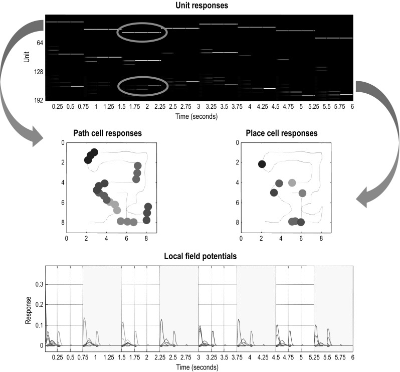
Fig. 7 Path and place cells: this figure revisits the simulation in Fig. 4 but focusing on the first 6 s of exploration. As in Fig. 4, the upper panel shows the simulated firing of the (192) units encoding expected hidden states, while the lower panel shows the accompanying local field potentials (obtained by band-pass filtering the neuronal activity in the upper panel). The key point made in this figure is that the first 64 units encode the location at the start of each local sequence of moves and maintain their firing until a subgoal has been reached. Conversely, the last 64 units encode the location at the end of the local sequence and therefore only fire after the accumulation of evidence that a subgoal has been reached. This leads to an asymmetry in the spatial temporal encoding of paths. In other words, the first set of units fire during short trajectories or paths to each subgoal, while the last set fire only when a particular (subgoal) location has been reached. This asymmetry is highlighted by circles in the upper panel (for the third subpath), which shows the first (upper) unit firing throughout the local sequence and the second (lower) unit firing only at the end. The resulting place preferences are illustrated in the middle panels, in terms of path cell (left panel) and place cell (right panel) responses. Here, we have indicated when the firing of selected units exceeds a threshold (of 0.8 Hz), as a function of location in the maze during exploration (the dotted red line). Each unit has been assigned a random colour. The key difference between path and place cell responses is immediately evident, path cells respond during short trajectories of paths through space, whereas place cell responses are elicited when, and only when, the corresponding place is visited (colour figure online)
Fig. 7 Path and place cells: this figure revisits the simulation in Fig. 4 but focusing on the first 6 s of exploration. As in Fig. 4, the upper panel shows the simulated firing of the (192) units encoding expected hidden states, while the lower panel shows the accompanying local field potentials (obtained by band-pass filtering the neuronal activity in the upper panel). The key point made in this figure is that the first 64 units encode the location at the start of each local sequence of moves and maintain their firing until a subgoal has been reached. Conversely, the last 64 units encode the location at the end of the local sequence and therefore only fire after the accumulation of evidence that a subgoal has been reached. This leads to an asymmetry in the spatial temporal encoding of paths. In other words, the first set of units fire during short trajectories or paths to each subgoal, while the last set fire only when a particular (subgoal) location has been reached. This asymmetry is highlighted by circles in the upper panel (for the third subpath), which shows the first (upper) unit firing throughout the local sequence and the second (lower) unit firing only at the end. The resulting place preferences are illustrated in the middle panels, in terms of path cell (left panel) and place cell (right panel) responses. Here, we have indicated when the firing of selected units exceeds a threshold (of 0.8 Hz), as a function of location in the maze during exploration (the dotted red line). Each unit has been assigned a random colour. The key difference between path and place cell responses is immediately evident, path cells respond during short trajectories of paths through space, whereas place cell responses are elicited when, and only when, the corresponding place is visited (colour figure online)CC BY · PubMed Central

Verification

Claims the paper makes

The claims and statistics of this paper haven’t been checked yet.

Free: it reads the open-access text and checks the first 5 claims that cite a source we can check. Create a free account to check every claim.

A few free checks a day · papers already verified open instantly · results are public

Claims other papers make about this one

Each is checked against this paper’s own text: does it say what the citing paper says it does?

Self-check

Percentages, sums and reported differences re-computed from the paper’s own numbers.

The self-check needs the paper’s full text.

Citations

Cites

Show all 98 references

Research works printed but not linked: 3

  1. Duff M (2002) Optimal learning: computational procedure for bayes-adaptive Markov decision processes. University of Massachusetts, Amherst
  2. Hartley T, Burgess N, Lever C, Cacucci F, O’Keefe J (2000) Modeling place fields in terms of the cortical inputs to the hippocampus. Hippocampus 10:369–379 · doi:10.1002/1098-1063(2000)10:4<369::aid-hipo3>3.0.co;2-0
  3. Sun Y, Gomez F, Schmidhuber J (2011b) Planning to be surprised: optimal Bayesian exploration in dynamic environments. In: Schmidhuber J et al (eds) Artificial general intelligence: 4th international conference, AGI 2011, Mountain View, CA, USA, August 3–6, 2011 Proceedings, pp 41–51. Springer, Berlin · DOI · Paper page

Cited by

See all 203

Metadata

Authors
Kaplan, R., & Friston, K. J.
Affiliations
Wellcome Centre for Human Neuroimaging (GB)
Corresponding author
Friston, Karl J.
Venue
Biological Cybernetics
Published
2018-03-23
Volume
112
Issue
4
Pages
323-343
ISSN
  • 0340-1200 (ISSN-L)
  • 1432-0770
OpenAlex
W2781668895
Cited by
203
References
98
Citations by year
2026: 12 · 2025: 22 · 2024: 29 · 2023: 27 · 2022: 34 · 2021: 36 · 2020: 28 · 2019: 10 · 2018: 5
FWCI
11.75
Type
journal article
Language
en
Open access
Licence
  • cc-by
  • creativecommons.org/licenses/by/4.0 (tdm)
Locations
  • Biological Cybernetics (publishedVersion, cc-by)
  • bioRxiv (Cold Spring Harbor Laboratory) (acceptedVersion, cc-by)
  • Europe PMC (PubMed Central) (publishedVersion, cc-by)
  • PubMed Central (publishedVersion, cc-by)
  • PubMed (publishedVersion)
  • UCL Discovery (University College London) (submittedVersion)
  • MPG.PuRe (Max Planck Society) (submittedVersion)
Funders
Wellcome Trust (088130/Z/09/Z)
Topics
  • Life Sciences › Neuroscience › Cognitive Neuroscience › Embodied and Extended Cognition
  • Life Sciences › Neuroscience › Cognitive Neuroscience › Memory and Neural Mechanisms
  • Physical Sciences › Computer Science › Artificial Intelligence › Reinforcement Learning in Robotics
Keywords
active inference, planning, navigation, free energy principle, uncertainty reduction, novelty, place cells, maze navigation, electrophysiological responses, goal-directed behavior
MeSH terms
Animals, Bayes Theorem, Brain, Computer Simulation, Goals, Humans, Models, Biological, Motivation, Neurons, Maze Learning, Spatial Navigation

About these checks

Registry, retraction, Cites and statistics results are computed, not judged, with one exception: a printed reference that no index lists is read once by a model before it counts as a citation error. Claims are extracted by a model and kept only when their quote appears verbatim in the text; each cited source is then checked, with a model’s help, for whether it says what the claim relies on. Those verdicts can be wrong — read the claim’s quote and the cited source before relying on one.

Statistics and arithmetic are recomputed, not judged.

Confidence bands are shown only for fields calibrated on our annotated test set. None is calibrated yet, so no band is shown.

What counts as a claim ›How we measure confidence ›How we check this ›

Are you an author, or do you see a problem with this page? Request a review

How to cite

Cite CoChat for the checks on this page, and the paper for its own findings.

This page
CoChat. (2026). Citation check: Planning and navigation as active inference. https://app.cochat.ai/papers/10.1007/s00422-018-0753-2
The paper
Kaplan, R., & Friston, K. J. (2018). Planning and navigation as active inference. Biological Cybernetics. https://doi.org/10.1007/s00422-018-0753-2

Data sources

Bibliographic data: Semantic Scholar, OpenAlex, Crossref.

Contains information from the Semantic Scholar Academic Graph Datasets, made available under the ODC Attribution License (ODC-BY 1.0).

Semantic Scholar’s data is described in: Kinney, R., et al. (2023). The Semantic Scholar Open Data Platform. arXiv:2301.10140.