

The DOI matches its Crossref record; 241 of the 241 references it cites were found in a registry or an index.
Mathematical framework for large-scale brain network modeling in The Virtual Brain
Open accessAbstract
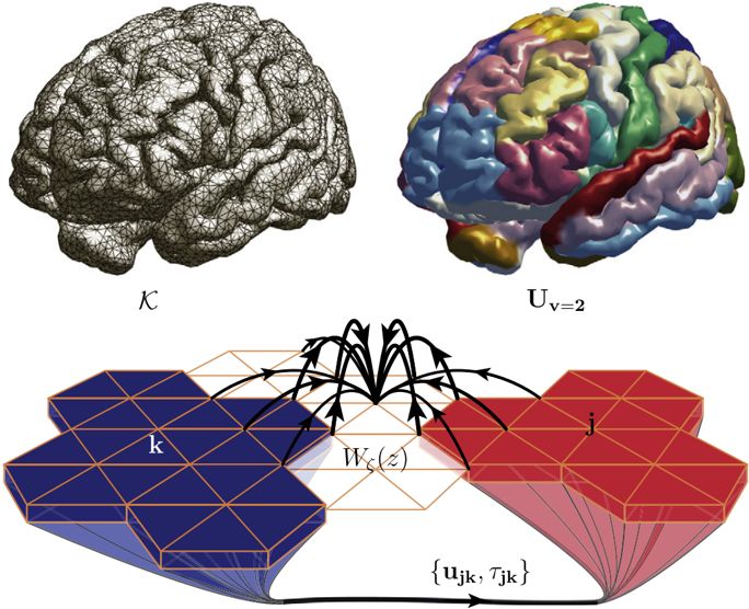
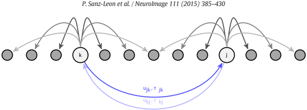
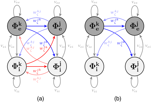
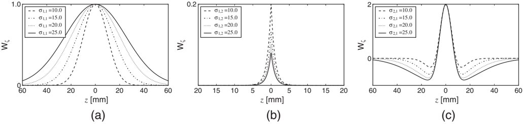
In this article, we describe the mathematical framework of the computational model at the core of the tool The Virtual Brain (TVB), designed to simulate collective whole brain dynamics by virtualizing brain structure and function, allowing simultaneous outputs of a number of experimental modalities such as electro- and magnetoencephalography (EEG, MEG) and functional Magnetic Resonance Imaging (fMRI). The implementation allows for a systematic exploration and manipulation of every underlying component of a large-scale brain network model (BNM), such as the neural mass model governing the local dynamics or the structural connectivity constraining the space time structure of the network couplings. Here, a consistent notation for the generalized BNM is given, so that in this form the equations represent a direct link between the mathematical description of BNMs and the components of the numerical implementation in TVB. Finally, we made a summary of the forward models implemented for mapping simulated neural activity (EEG, MEG, sterotactic electroencephalogram (sEEG), fMRI), identifying their advantages and limitations.
Overview
The claims and statistics of this paper haven’t been checked yet.
Run the check — free, no account needed. It reads the open-access text and checks the sources it cites.
Integrity signals
Registry
Cites
Statistics
Figures
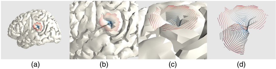
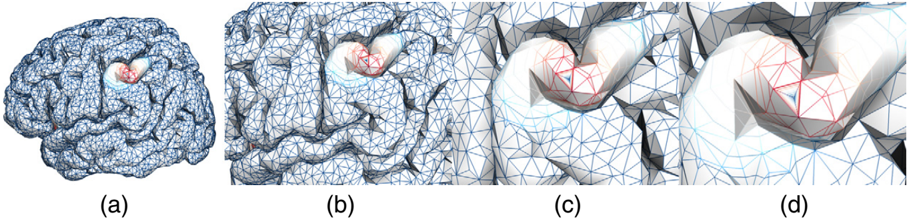
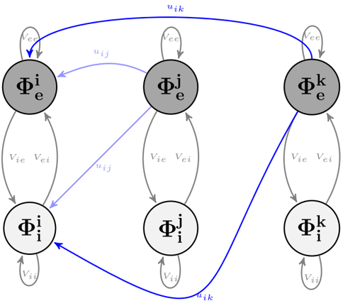
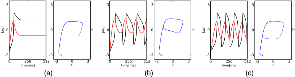
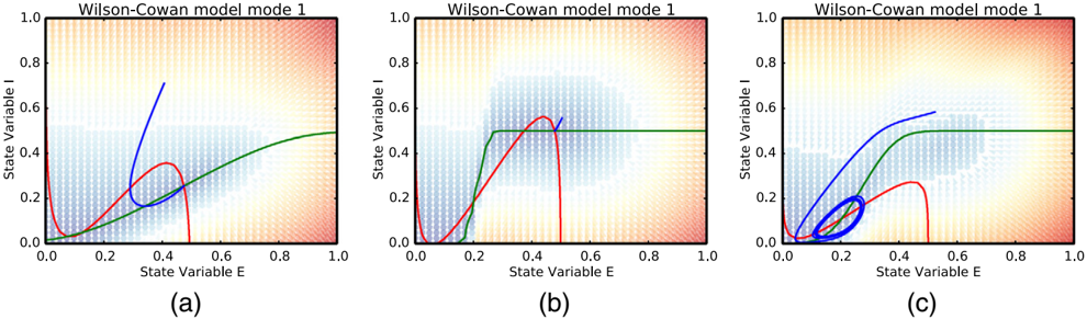
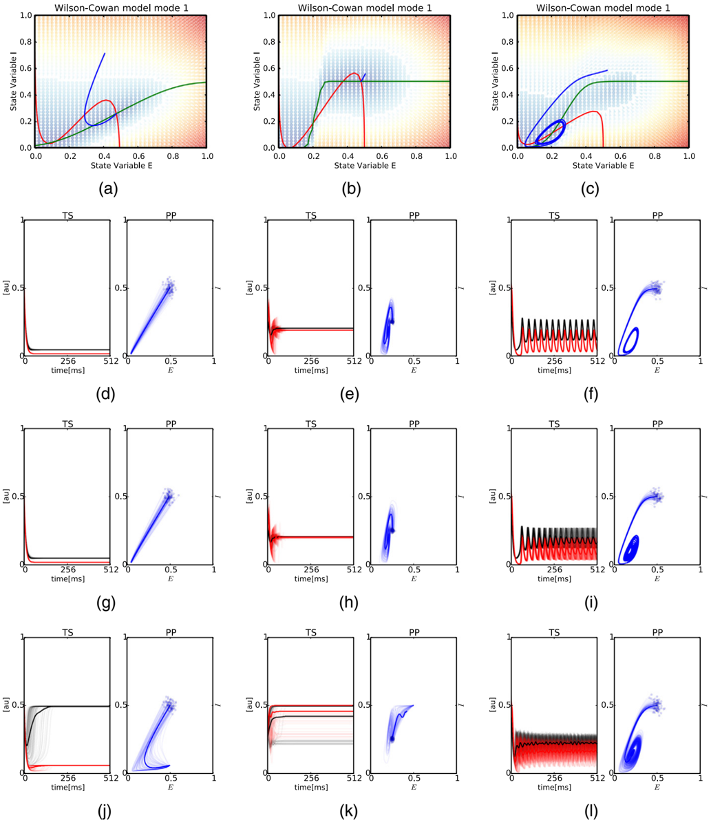
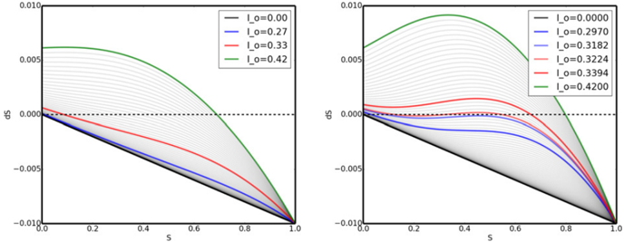
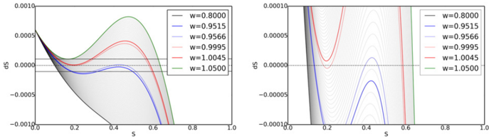
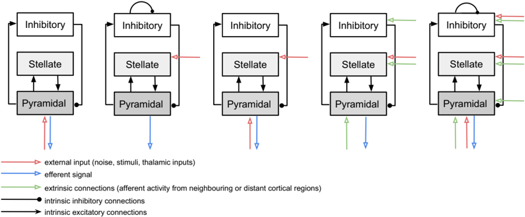
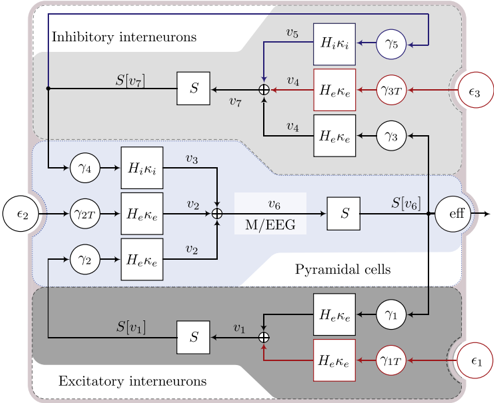
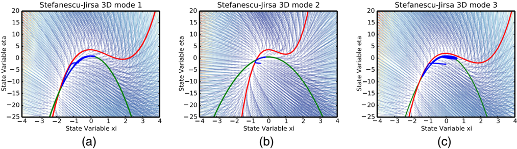
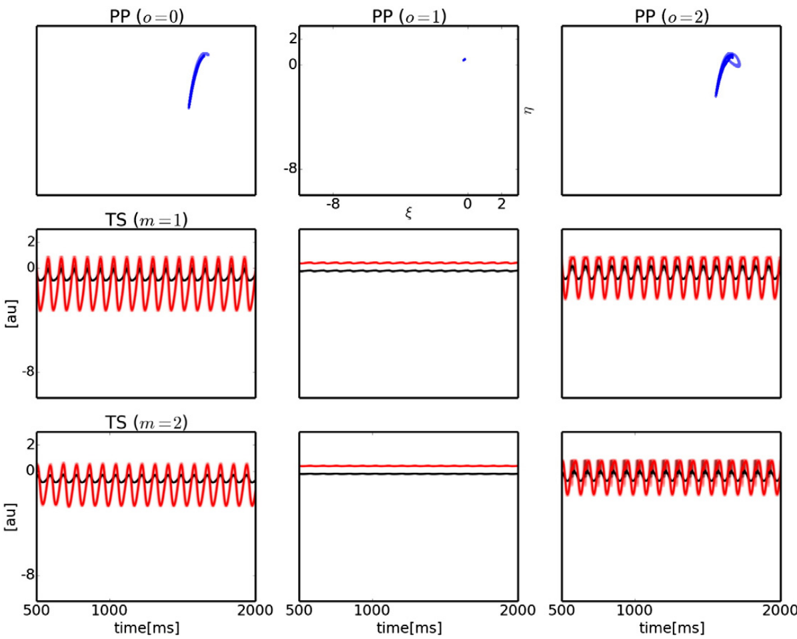
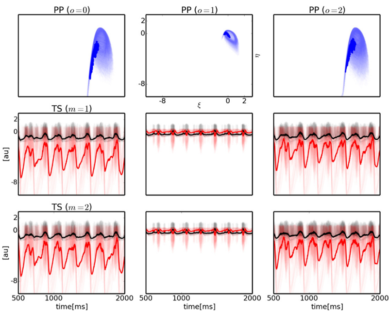
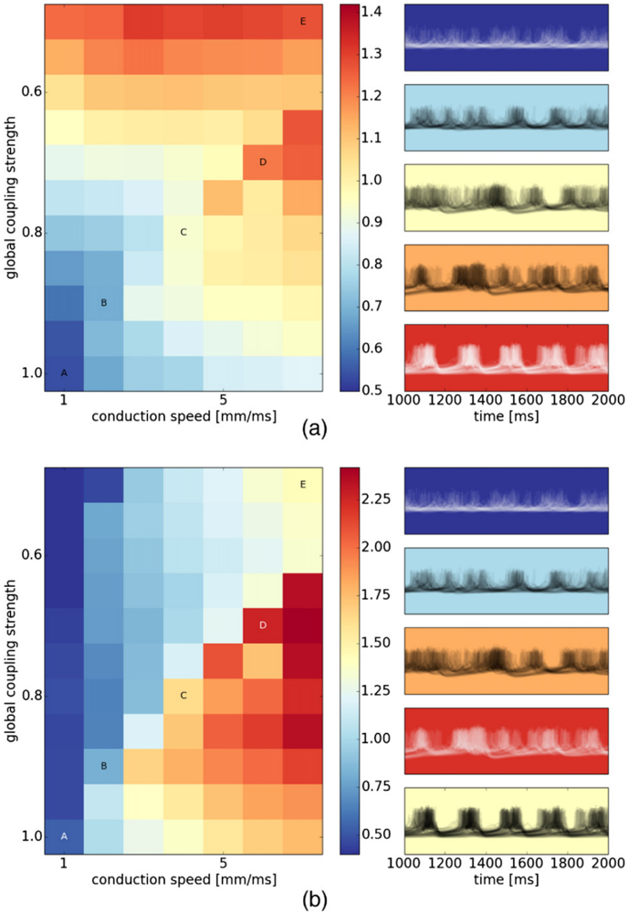
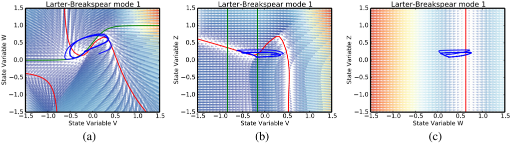
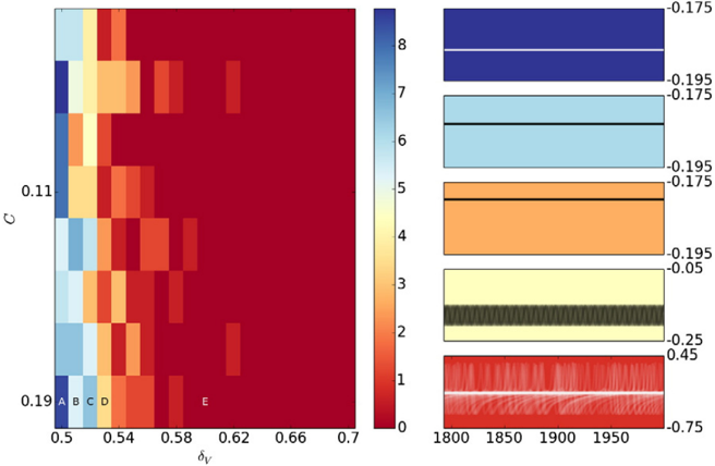
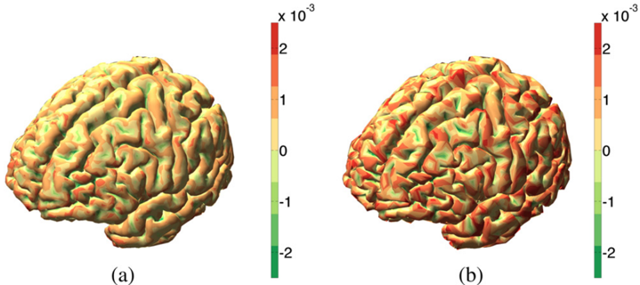
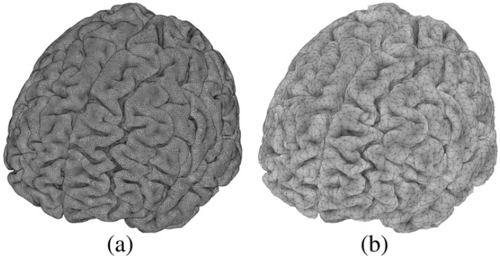
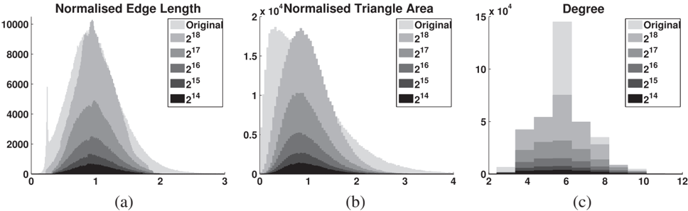
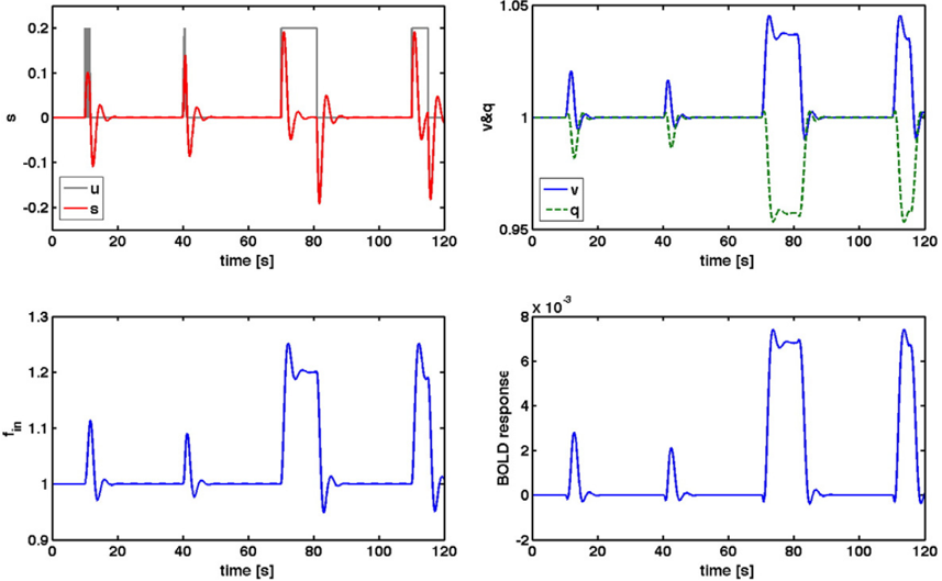
Verification
Claims the paper makes
The claims and statistics of this paper haven’t been checked yet.
Run the check — free, no account needed. It reads the open-access text and checks the sources it cites.
Claims other papers make about this one
Each is checked against this paper’s own text: does it say what the citing paper says it does?
In the citing paper
“Models can involve highly parameterized simulations of regional activity (Hansen et al., 2015; Messe et al., 2014; Sanz-Leon et al., 2015), or sparser analytic predictions of FC using graph metrics of mutual communication (Goni et al., 2014; Grayson et al., 2016) (although, both approaches appear to be comparably effective; see Figure 1D).”
From Development of large-scale functional networks from birth to adulthood: A guide to the neuroimaging literature (2017) · cites this paper as Sanz-Leon et al., 2015
Self-check
Percentages, sums and reported differences re-computed from the paper’s own numbers.
The self-check needs the paper’s full text.
Citations
Cites
Tzourio-Mazoyer, N., Landeau, B., Papathanassiou, D., Crivello, F., Etard, O., Delcroix, N., Mazoyer, B., & Joliot, M. (2002) · NeuroImage · doi:10.1006/nimg.2001.0978 · Cited by 16,319
Desikan, R. S., Ségonne, F., Fischl, B., Quinn, B. T., Dickerson, B. C., Blacker, D., Buckner, R. L., Dale, A. M., Maguire, R. P., Hyman, B. T., et al. (2006) · NeuroImage · doi:10.1016/j.neuroimage.2006.01.021 · Cited by 13,324
Cortical Surface-Based Analysis
Dale, A. M., Fischl, B., & Sereno, M. I. (1999) · NeuroImage · doi:10.1006/nimg.1998.0395 · Cited by 10,910
Oostenveld, R., Fries, P., Maris, E., & Schoffelen, J.-M. (2011) · Computational Intelligence and Neuroscience · doi:10.1155/2011/156869 · Cited by 10,323
Functional connectivity in the motor cortex of resting human brain using echo‐planar mri
Biswal, B., Zerrin Yetkin, F., Haughton, V. M., & Hyde, J. S. (1995) · Magnetic Resonance in Medicine · doi:10.1002/mrm.1910340409 · Cited by 9,812
Statistical parametric maps in functional imaging: A general linear approach
Friston, K. J., Holmes, A. P., Worsley, K. J., Poline, J. ‐., Frith, C. D., & Frackowiak, R. S. J. (1994) · Human Brain Mapping · doi:10.1002/hbm.460020402 · Cited by 9,688
The organization of the human cerebral cortex estimated by intrinsic functional connectivity
Thomas Yeo, B. T., Krienen, F. M., Sepulcre, J., Sabuncu, M. R., Lashkari, D., Hollinshead, M., Roffman, J. L., Smoller, J. W., Zöllei, L., Polimeni, J. R., et al. (2011) · Journal of Neurophysiology · doi:10.1152/jn.00338.2011 · Cited by 9,182
The organization of the human cerebellum estimated by intrinsic functional connectivity
Buckner, R. L., Krienen, F. M., Castellanos, A., Diaz, J. C., & Yeo, B. T. T. (2011) · Journal of Neurophysiology · doi:10.1152/jn.00339.2011 · Cited by 7,304
Spontaneous fluctuations in brain activity observed with functional magnetic resonance imaging
Fox, M. D., & Raichle, M. E. (2007) · Nature Reviews Neuroscience · doi:10.1038/nrn2201 · Cited by 6,700
Brain magnetic resonance imaging with contrast dependent on blood oxygenation.
Ogawa, S., Lee, T. M., Kay, A. R., & Tank, D. W. (1990) · Proceedings of the National Academy of Sciences · doi:10.1073/pnas.87.24.9868 · Cited by 6,483
Research works printed but not linked: 1
- Spiegler, 2015, The critical brain: dissipation and restin-state networks, PNAS
Cited by
Sorted by citations
The Kuramoto model in complex networks
Rodrigues, F. A., Peron, T., Ji, P., & Kurths, J. (2015) · Physics Reports · doi:10.1016/j.physrep.2015.10.008 · Cited by 1,064
“Other recent works have investigated further aspects of the relation between structure and dynamics of phase oscillators in anatomical and functional cortical networks [214, 378, 401–406], which includes studies on the effects of remote synchronization [407–409], a toolbox for large-scale simulations of brain dynamics…”
BackgroundLinking Structure and Function in Macroscale Brain Networks
Suárez, L. E., Markello, R. D., Betzel, R. F., & Mišić, B. (2020) · Trends in Cognitive Sciences · doi:10.1016/j.tics.2020.01.008 · Cited by 769
Gradients of structure–function tethering across neocortex
Vázquez-Rodríguez, B., Suárez, L. E., Markello, R. D., Shafiei, G., Paquola, C., Hagmann, P., van den Heuvel, M. P., Bernhardt, B. C., Spreng, R. N., & Mišić, B. (2019) · Proceedings of the National Academy of Sciences · doi:10.1073/pnas.1903403116 · Cited by 472
Grayson, D. S., & Fair, D. A. (2017) · NeuroImage · doi:10.1016/j.neuroimage.2017.01.079 · Cited by 411
“Given that macroscale FC is modulated by both interregional connectivity strength as well as local population dynamics (Sanz-Leon et al., 2015), alterations in SC-FC coupling could potentially point to important shifts in the underlying drivers of various network phenomena.”
BackgroundThe Virtual Epileptic Patient: Individualized whole-brain models of epilepsy spread
Jirsa, V., Proix, T., Perdikis, D., Woodman, M., Wang, H., Gonzalez-Martinez, J. A., Bernard, C., Bénar, C., Guye, M., Chauvel, P., et al. (2016) · NeuroImage · doi:10.1016/j.neuroimage.2016.04.049 · Cited by 435
Self-citationIndividual brain structure and modelling predict seizure propagation
Proix, T., Bartoloméi, F., Guye, M., & Jirsa, V. (2017) · Brain · doi:10.1093/brain/awx004 · Cited by 286
“A BNM (Sanz-Leon et al., 2015) was constructed by placing at each node of the parcellation a neural mass model able to reproduce the temporal seizure dynamics and to switch autonomously between interictal and ictal states, the so-called Epileptor model (Jirsa et al., 2014).”
MethodSelf-citationComputational models of epileptiform activity
Wendling, F., Benquet, P., Bartoloméi, F., & Jirsa, V. (2015) · Journal of Neuroscience Methods · doi:10.1016/j.jneumeth.2015.03.027 · Cited by 199
Self-citationInferring multi-scale neural mechanisms with brain network modelling
Schirner, M., McIntosh, A. R., Jirsa, V., Deco, G., & Ritter, P. (2018) · eLife · doi:10.7554/elife.28927 · Cited by 204
Self-citationTranslational perspectives for computational neuroimaging
Stephan, K. E., Iglesias, S., Heinzle, J., & Diaconescu, A. O. (2015) · Neuron · doi:10.1016/j.neuron.2015.07.008 · Cited by 169
“A notable example of the rapid development of large-scale BNMs for neuroimaging data is the ‘‘Virtual Brain’’ project (Jirsa et al., 2010; Sanz-Leon et al., 2015).”
BackgroundLocal structure-function relationships in human brain networks across the lifespan
Esfahlani, F. Z., Faskowitz, J., Slack, J., Mišić, B., & Betzel, R. F. (2022) · Nature Communications · doi:10.1038/s41467-022-29770-y · Cited by 178
Frässle, S., Lomakina, E. I., Razi, A., Friston, K. J., Buhmann, J. M., & Stephan, K. E. (2017) · NeuroImage · doi:10.1016/j.neuroimage.2017.02.090 · Cited by 163
Kunze, T., Hunold, A., Haueisen, J., Jirsa, V., & Spiegler, A. (2016) · NeuroImage · doi:10.1016/j.neuroimage.2016.02.015 · Cited by 162
“The time course of uPy(t) of each area constituted the output of each area in the network and was propagated to a set of 62 EEG sensors by means of a propagation matrix, which was already included in the according TVB dataset.”
MethodInfluentialSelf-citationMagnetoencephalography in Cognitive Neuroscience: A Primer
Groß, J. (2019) · Neuron · doi:10.1016/j.neuron.2019.07.001 · Cited by 177
“One example of this approach is implemented in the Virtual Brain software (https://thevirtualbrain.org/tvb/zwei; Deco et al., 2017; Sanz-Leon et al., 2015; Schirner et al., 2018).”
MethodThe quest for multiscale brain modeling
D'Angelo, E. U., & Jirsa, V. (2022) · Trends in Neurosciences · doi:10.1016/j.tins.2022.06.007 · Cited by 162
Self-citationProix, T., Jirsa, V., Bartoloméi, F., et al. (2018) · Nature Communications · doi:10.1038/s41467-018-02973-y · Cited by 152
“Mixed connectivities in network architectures are common in large-scale brain models 39,40 .”
Self-citationAn automated pipeline for constructing personalized virtual brains from multimodal neuroimaging data
Schirner, M., Rothmeier, S., Jirsa, V., McIntosh, A. R., & Ritter, P. (2015) · NeuroImage · doi:10.1016/j.neuroimage.2015.03.055 · Cited by 147
Self-citationMapping how local perturbations influence systems-level brain dynamics
Gollo, L. L., Roberts, J. A., & Cocchi, L. (2017) · NeuroImage · doi:10.1016/j.neuroimage.2017.01.057 · Cited by 144
“Mean-field models at the whole-brain scale roughly fall into two categories: coupled neural masses (Gollo and Breakspear, 2014; Sanz-Leon et al., 2015; Schmidt et al., 2015) and neural fields (Atasoy et al., 2016; Jirsa and Haken, 1996; Robinson et al., 2001; Robinson et al., 2016).”
BackgroundStefanovski, L., Triebkorn, P., Spiegler, A., Díaz-Cortés, M.-A., Solodkin, A., Jirsa, V., McIntosh, A. R., Ritter, P., & Initiative, A. D. N. (2019) · Frontiers in Computational Neuroscience · doi:10.3389/fncom.2019.00054 · Cited by 145
Self-citationLearning function from structure in neuromorphic networks
Suárez, L. E., Richards, B. A., Lajoie, G., & Mišić, B. (2021) · Nature Machine Intelligence · doi:10.1038/s42256-021-00376-1 · Cited by 137
Iturria‐Medina, Y., Carbonell, F., Sotero, R. C., Chouinard-Decorte, F., & Evans, A. C. (2017) · NeuroImage · doi:10.1016/j.neuroimage.2017.02.058 · Cited by 130
“…to take action locally and spread through anatomical connections (Cabral et al., 2012; Friston et al., 2014; Iturria-Medina et al., 2014; Mišić et al., 2015; Raj et al., 2012; Sanz Leon et al., 2013; Sanz-Leon et al., 2015; Sotero et al., 2007; Stam et al., 2016; Valdes-sosa et al., 2011a).”
Transmission time delays organize the brain network synchronization
Petkoski, S., & Jirsa, V. (2019) · Philosophical Transactions of the Royal Society A Mathematical Physical and Engineering Sciences · doi:10.1098/rsta.2018.0132 · Cited by 137
Self-citationHashemi, M., Vattikonda, A. N., Ší́p, V., Guye, M., Bartoloméi, F., Woodman, M., & Jirsa, V. (2020) · NeuroImage · doi:10.1016/j.neuroimage.2020.116839 · Cited by 123
Self-citationSymmetry Breaking in Space-Time Hierarchies Shapes Brain Dynamics and Behavior
Pillai, A. S., & Jirsa, V. (2017) · Neuron · doi:10.1016/j.neuron.2017.05.013 · Cited by 132
Self-citationWang, H., Woodman, M., Triebkorn, P., Lemaréchal, J.-D., Jha, J., Dollomaja, B., Vattikonda, A. N., Ší́p, V., Villalon, S. M., Hashemi, M., et al. (2023) · Science Translational Medicine · doi:10.1126/scitranslmed.abp8982 · Cited by 117
“The Virtual Brain (TVB) ( 8 ) is a neuroinfor-matics platform for the construction and simulation of virtual brains that can provide the required functionality for EZN estimation and make it possible to perform causal inference on the full brain scale.”
MethodInfluentialSelf-citationBrain simulation as a cloud service: The Virtual Brain on EBRAINS
Schirner, M., Domide, L., Perdikis, D., Triebkorn, P., Stefanovski, L., Pai, R. K., Prodan, P., Valean, B., Palmer, J., Langford, C., et al. (2022) · NeuroImage · doi:10.1016/j.neuroimage.2022.118973 · Cited by 127
Self-citationVirtual brain twins: from basic neuroscience to clinical use
Wang, H., Triebkorn, P., Breyton, M., Dollomaja, B., Lemaréchal, J.-D., Petkoski, S., Sorrentino, P., Depannemaecker, D., Hashemi, M., & Jirsa, V. (2024) · National Science Review · doi:10.1093/nsr/nwae079 · Cited by 127
Self-citationEdges in brain networks: Contributions to models of structure and function
Faskowitz, J., Betzel, R. F., & Sporns, O. (2021) · Network Neuroscience · doi:10.1162/netn_a_00204 · Cited by 110
Zimmermann, J., Perry, A., Breakspear, M. J., Schirner, M., Sachdev, P. S., Wen, W., Kochan, N. A., Mapstone, M., Ritter, P., McIntosh, A. R., et al. (2018) · NeuroImage Clinical · doi:10.1016/j.nicl.2018.04.017 · Cited by 102
Brain-Inspired Computing: A Systematic Survey and Future Trends
Li, G., Deng, L., Tang, H., Pan, G., Tian, Y., Roy, K., & Maass, W. (2024) · Proceedings of the IEEE · doi:10.1109/jproc.2024.3429360 · Cited by 113
“…to macroscopic scale (e.g., mean-field neural mass models of brain regions [384], [385], and models of entire brain networks [124], [386], [387]), and new properties persistently emerge and previous properties may vanish during the cross-scale transmission of neural dynamics, which can be…”
CoreNEURON : An Optimized Compute Engine for the NEURON Simulator
Kumbhar, P., Hines, M. L., FOURIAUX, J., Ovcharenko, A., King, J. G., Delalondre, F., & Schürmann, F. (2019) · Frontiers in Neuroinformatics · doi:10.3389/fninf.2019.00063 · Cited by 98
Next-generation neural mass and field modeling
Byrne, Á., O’Dea, R. D., Forrester, M., Ross, J., & Coombes, S. (2019) · Journal of Neurophysiology · doi:10.1152/jn.00406.2019 · Cited by 101
“Moreover, Wilson–Cowan style neural mass models are a key component of the Virtual Brain project that aims to deliver the first simulation of the human brain based on personalised large-scale connectivity [105].”
BackgroundSpiegler, A., Hansen, E. C. A., Bernard, C., McIntosh, A. R., & Jirsa, V. (2016) · eNeuro · doi:10.1523/eneuro.0068-16.2016 · Cited by 96
Self-citationIndividual structural features constrain the mouse functional connectome
Melozzi, F., Bergmann, E., Harris, J. A., Kahn, I., Jirsa, V., & Bernard, C. (2019) · Proceedings of the National Academy of Sciences · doi:10.1073/pnas.1906694116 · Cited by 89
Self-citationNeuronal Cascades Shape Whole-Brain Functional Dynamics at Rest
Rabuffo, G., Fousek, J., Bernard, C., & Jirsa, V. (2021) · eNeuro · doi:10.1523/eneuro.0283-21.2021 · Cited by 91
“36 We use The Virtual Brain (TVB), a neuroinformatics and simulation platform, which allows 37 connectome-based whole brain modeling of multiple species including human [28] and mice [29].”
MethodSelf-citationDynamical Mechanisms of Interictal Resting-State Functional Connectivity in Epilepsy
Courtiol, J., Guye, M., Bartoloméi, F., Petkoski, S., & Jirsa, V. (2020) · Journal of Neuroscience · doi:10.1523/jneurosci.0905-19.2020 · Cited by 85
Self-citationVirtual epileptic patient brain modeling: Relationships with seizure onset and surgical outcome
Makhalova, J., Villalon, S. M., Wang, H., et al. (2022) · Epilepsia · doi:10.1111/epi.17310 · Cited by 85
Self-citationNext Generation Neural Mass Models
Coombes, S., & Byrne, Á. (2018) · PoliTO Springer series · doi:10.1007/978-3-319-71048-8_1 · Cited by 84
“Moreover, they are now an integral part of the Virtual Brain project that aims to deliver the first open simulation of the human brain based on individual large-scale connectivity [14], as well as play a key role in the neurocomputational modelling of neurological and psychiatric disorders [15].”
BackgroundBiophysically detailed forward modeling of the neural origin of EEG and MEG signals
Næss, S., Halnes, G., Hagen, E., Hagler, D. J., Dale, A. M., Einevoll, G. T., & Ness, T. V. (2021) · NeuroImage · doi:10.1016/j.neuroimage.2020.117467 · Cited by 66
Clinical Concepts Emerging from fMRI Functional Connectomics
Matthews, P. M., & Hampshire, A. (2016) · Neuron · doi:10.1016/j.neuron.2016.07.031 · Cited by 83
“, The Virtual Brain (Sanz-Leon et al., 2015), the Blue Brain Project (Markram et al.”
Proix, T., Spiegler, A., Schirner, M., Rothmeier, S., Ritter, P., & Jirsa, V. (2016) · NeuroImage · doi:10.1016/j.neuroimage.2016.06.016 · Cited by 86
“…(BNMs) are networks of neural masses that can provide a first order approximation to explain such brain signals (Bojak and Oostendorp, 2011; Deco et al., 2009; Deco and Jirsa, 2012; Ghosh et al., 2008; Jirsa et al., 2010; Ritter et al., 2013; Sanz-Leon et al., 2015; Spiegler and Jirsa, 2013).”
BackgroundMethodInfluentialSelf-citationPersonalized brain network models for assessing structure–function relationships
Bansal, K., Nakuci, J., & Muldoon, S. F. (2018) · Current Opinion in Neurobiology · doi:10.1016/j.conb.2018.04.014 · Cited by 81
Batallé, D., Edwards, A. D., & O’Muircheartaigh, J. (2017) · Journal of Child Psychology and Psychiatry · doi:10.1111/jcpp.12838 · Cited by 92
A macaque connectome for large-scale network simulations in TheVirtualBrain
Shen, K., Bezgin, G., Schirner, M., Ritter, P., Everling, S., & McIntosh, A. R. (2019) · Scientific Data · doi:10.1038/s41597-019-0129-z · Cited by 78
Petkoski, S., Palva, J. M., & Jirsa, V. (2018) · PLoS Computational Biology · doi:10.1371/journal.pcbi.1006160 · Cited by 88
Self-citationMultistability in Large Scale Models of Brain Activity
Golos, M., Jirsa, V., & Daucé, E. (2015) · PLoS Computational Biology · doi:10.1371/journal.pcbi.1004644 · Cited by 80
Self-citationArtificial Intelligence and Computational Approaches for Epilepsy
An, S., Kang, C., & Lee, H. W. (2020) · Journal of Epilepsy Research · doi:10.14581/jer.20003 · Cited by 75
“They have proposed a novel methodology to develop individual brain network models, so called the Virtual Epileptic Patient (VEP),(98) by incorporating multimodal data from each epilepsy patient, and have also developed and distributed the neuroinformatics platform, The Virtual Brain, to enable the model construction.(…”
MethodFunctional Mechanisms of Recovery after Chronic Stroke: Modeling with the Virtual Brain
Falcon, M. I., Riley, J. D., Jirsa, V., McIntosh, A. R., Chen, E. E., & Solodkin, A. (2016) · eNeuro · doi:10.1523/eneuro.0158-15.2016 · Cited by 70
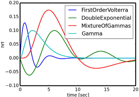
“…of the system was performed using stochastic Heun’s method (Mannella 2002), with an integration step size of 0.0122 ms. (5) The BOLD signals were derived from the field potentials using a hemodynamic response function implemented with a gamma kernel (Boynton et al., 1996; Sanz-Leon et al., 2015).”
InfluentialSelf-citationFitzgibbon, S. P., DeLosAngeles, D., Lewis, T. W., Powers, D. M. W., Grummett, T. S., Whitham, E. M., Ward, L. M., Willoughby, J. O., & Pope, K. J. (2015) · Clinical Neurophysiology · doi:10.1016/j.clinph.2015.12.009 · Cited by 67
The Digital Twin Brain: A Bridge between Biological and Artificial Intelligence
Xiong, H., Chu, C., Fan, L., Song, M. X., Zhang, J., Ma, Y., Zheng, R., Zhang, J., Yang, Z., & Jiang, T. (2023) · Intelligent Computing · doi:10.34133/icomputing.0055 · Cited by 69
Modeling regional changes in dynamic stability during sleep and wakefulness
Ipiña, I. P., Kehoe, P. D., Kringelbach, M. L., Laufs, H., Ibáñez, A. M., Deco, G., Perl, Y. S., & Tagliazucchi, E. (2020) · NeuroImage · doi:10.1016/j.neuroimage.2020.116833 · Cited by 67
Luppi, A. I., Mediano, P. A. M., Rosas, F. E., Allanson, J. E., Pickard, J. D., Williams, G. B., Craig, M. M., Finoia, P., Peattie, A. R. D., Coppola, P., et al. (2022) · Communications Biology · doi:10.1038/s42003-022-03330-y · Cited by 79
On the central role of brain connectivity in neurodegenerative disease progression
Iturria‐Medina, Y., & Evans, A. C. (2015) · Frontiers in Aging Neuroscience · doi:10.3389/fnagi.2015.00090 · Cited by 62
“Similarly, there are promising advances in the modeling and understanding of neuronal/synaptic spreading across structural networks (Sotero et al., 2007; Valdes-Sosa et al., 2009; Sanz-Leon et al., 2013, 2015; Messé et al., 2015), but thesemethodologies also require additional predictive validation.”
BackgroundPutting the “dynamic” back into dynamic functional connectivity
Heitmann, S., & Breakspear, M. J. (2018) · Network Neuroscience · doi:10.1162/netn_a_00041 · Cited by 65
Melozzi, F., Woodman, M., Jirsa, V., & Bernard, C. (2017) · eNeuro · doi:10.1523/eneuro.0111-17.2017 · Cited by 68
“, 2000) using the default value implemented in The Virtual Brain (Sanz-Leon et al., 2015).”
BackgroundMethodInfluentialSelf-citationSrivastava, P., Nozari, E., Kim, J. Z., Ju, H., Zhou, D., Becker, C. O., Pasqualetti, F., Pappas, G. J., & Bassett, D. S. (2020) · Network Neuroscience · doi:10.1162/netn_a_00158 · Cited by 65
It’s about time: Linking dynamical systems with human neuroimaging to understand the brain
John, Y. J., Sawyer, K. S., Srinivasan, K., Müller, E. J., Munn, B., & Shine, J. M. (2022) · Network Neuroscience · doi:10.1162/netn_a_00230 · Cited by 71
“The Virtual Brain (Ritter et al., 2013; Sanz-Leon et al., 2015; Schirner et al., 2021) is an excellent example of a toolbox that affords access to this approach, and has been used to demonstrate important links between structure and function across many spatiotemporal scales.”
MethodA comprehensive neural simulation of slow-wave sleep and highly responsive wakefulness dynamics
Goldman, J. S., Kusch, L., Aquilué-Llorens, D., Yalçınkaya, B. H., Depannemaecker, D., Ancourt, K., Nghiem, T.-A. E., Jirsa, V., & Alain Destexhe, A. (2023) · Frontiers in Computational Neuroscience · doi:10.3389/fncom.2022.1058957 · Cited by 65
Self-citationLawn, T., Howard, M. A., Turkheimer, F., Mišić, B., Deco, G., Martins, D., & Dipasquale, O. (2023) · Neuroscience & Biobehavioral Reviews · doi:10.1016/j.neubiorev.2023.105193 · Cited by 64
“(Ritter et al., 2013; Sanz-Leon et al., 2015) to model the perturbed network dynamics seen in patients with Alzheimer’s disease (Stefanovski et al.”
A new neuroinformatics approach to personalized medicine in neurology: The Virtual Brain
Falcon, M. I., Jirsa, V., & Solodkin, A. (2016) · Current Opinion in Neurology · doi:10.1097/wco.0000000000000344 · Cited by 59
Self-citationHeterogeneity of time delays determines synchronization of coupled oscillators
Petkoski, S., Spiegler, A., Proix, T., Aram, P., Temprado, J.-J., & Jirsa, V. (2016) · Physical review. E · doi:10.1103/physreve.94.012209 · Cited by 61
Self-citationModel-based whole-brain effective connectivity to study distributed cognition in health and disease
Gilson, M., Zamora‐López, G., Pallarés, V., Adhikari, M. H., Senden, M., Campo, A. T., Mantini, D., Corbetta, M., Deco, G., & Insabato, A. (2019) · Network Neuroscience · doi:10.1162/netn_a_00117 · Cited by 62
Multiscale modeling of brain dynamics: from single neurons and networks to mathematical tools
Siettos, C. I., & Starke, J. (2016) · WIREs Systems Biology and Medicine · doi:10.1002/wsbm.1348 · Cited by 58
Becker, R., Knock, S. A., Ritter, P., & Jirsa, V. (2015) · PLoS Computational Biology · doi:10.1371/journal.pcbi.1004352 · Cited by 53
Self-citationKuramoto Model for Excitation-Inhibition-Based Oscillations
Montbrió, E., & Pazó, D. (2018) · Physical Review Letters · doi:10.1103/physrevlett.120.244101 · Cited by 57
Papadopoulos, L., Lynn, C. W., Battaglia, D. A., & Bassett, D. S. (2020) · PLoS Computational Biology · doi:10.1371/journal.pcbi.1008144 · Cited by 54
NFTsim: Theory and Simulation of Multiscale Neural Field Dynamics
Sanz‐Leon, P., Robinson, P. A., Knock, S. A., Drysdale, P. M., Abeysuriya, R., Fung, F., RENNIE, C. J., & Zhao, X. (2018) · PLoS Computational Biology · doi:10.1371/journal.pcbi.1006387 · Cited by 57
“125 A few software packages are available to model neural masses and neural fields: [7] 126 developed a neuroinformatics platform for large-scale brain modeling in terms of a 127 network of linked neural masses with anatomically specified cortical geometry [55], 128 long-range connectivity, and local short-range conne…”
BackgroundMethodSelf-citationThe Virtual Brain: Modeling Biological Correlates of Recovery after Chronic Stroke
Falcon, M. I., Riley, J. D., Jirsa, V., McIntosh, A. R., Shereen, A. D., Chen, E. E., & Solodkin, A. (2015) · Frontiers in Neurology · doi:10.3389/fneur.2015.00228 · Cited by 54
Self-citationHashemi, M., Vattikonda, A. N., Jha, J., Ší́p, V., Woodman, M., Bartoloméi, F., & Jirsa, V. (2023) · Neural Networks · doi:10.1016/j.neunet.2023.03.040 · Cited by 52
Self-citationPartial synchronization patterns in brain networks
Schöll, E. (2021) · Europhysics Letters (EPL) · doi:10.1209/0295-5075/ac3b97 · Cited by 50
Tesler, F., Linne, M., & Alain Destexhe, A. (2023) · Scientific Reports · doi:10.1038/s41598-023-32618-0 · Cited by 47
“Furthermore, our framework can be combined with different neuronal models and has the potential of being incorporated in whole brain simulators such as The Virtual Brain 44,69 .”
MethodYu, Y., Fan, Y., Han, F., Luan, G., & Wang, Q. (2023) · Science China Technological Sciences · doi:10.1007/s11431-022-2341-x · Cited by 49
Stefanovski, L., Meier, J. M., Pai, R. K., Triebkorn, P., Lett, T. A. P., Martin, L., Bülau, K., Hofmann‐Apitius, M., Solodkin, A., McIntosh, A. R., et al. (2021) · Frontiers in Neuroinformatics · doi:10.3389/fninf.2021.630172 · Cited by 47
Synchronization patterns: from network motifs to hierarchical networks
Krishnagopal, S., Lehnert, J., Poel, W., Zakharova, A., & Schöll, E. (2017) · Philosophical Transactions of the Royal Society A Mathematical Physical and Engineering Sciences · doi:10.1098/rsta.2016.0216 · Cited by 45
Dubois, J., Adibpour, P., Poupon, C., Hertz-Pannier, L., & Dehaene-Lambertz, G. (2016) · Brain Plasticity · doi:10.3233/bpl-160031 · Cited by 40
“Thus accurate anatomo-functional models of networks would require to integer all these properties and account for spatial and temporal constraints [150].”
BackgroundArbabyazd, L., Shen, K., Wang, Z., Hofmann‐Apitius, M., Ritter, P., McIntosh, A. R., Battaglia, D. A., & Jirsa, V. (2021) · eNeuro · doi:10.1523/eneuro.0475-20.2021 · Cited by 44
Self-citationDoes the brain behave like a (complex) network? I. Dynamics
Papo, D., & Buldú, J. M. (2023) · Physics of Life Reviews · doi:10.1016/j.plrev.2023.12.006 · Cited by 44
Data-driven brain network models differentiate variability across language tasks
Bansal, K., Medaglia, J. D., Bassett, D. S., Vettel, J. M., & Muldoon, S. F. (2018) · PLoS Computational Biology · doi:10.1371/journal.pcbi.1006487 · Cited by 42
“Using experimentally obtained structural brain network data combined with biologically motivated computational models of brain dynamics [36], one can build personalized brain network models of human brain activity [37, 38, 39].”
MethodHashemi, M., Vattikonda, A. N., Ší́p, V., Diaz-Pier, S., Peyser, A., Wang, H., Guye, M., Bartoloméi, F., Woodman, M., & Jirsa, V. (2021) · PLoS Computational Biology · doi:10.1371/journal.pcbi.1009129 · Cited by 39
“The Virtual Brain (TVB) is a computational framework to simulate large-scale brain network models based on individual subject data [59, 60].”
BackgroundSelf-citationStructural and functional, empirical and modeled connectivity in the cerebral cortex of the rat
Díaz‐Parra, A., Osborn, Z. G., Canals, S., Moratal, D., & Sporns, O. (2017) · NeuroImage · doi:10.1016/j.neuroimage.2017.07.046 · Cited by 41
“TVB simulations take structural data about a brain - structural connectivity, spatial coordinates of ROIs, and tract length distances between ROIs - and output simulated neural activity time series for each ROI, using a given model type and set of simulation parameter values (Sanz-Leon et al., 2015).”
MethodIturria‐Medina, Y., Carbonell, F., & Evans, A. C. (2018) · NeuroImage · doi:10.1016/j.neuroimage.2018.06.028 · Cited by 42
Mean-Field Models for EEG/MEG: From Oscillations to Waves
Byrne, Á., Ross, J., Nicks, R., & Coombes, S. (2021) · Brain Topography · doi:10.1007/s10548-021-00842-4 · Cited by 42
“2020), and are a key ingredient of the Virtual Brain project that aims to deliver the first open simulation of the human brain based on individual large-scale connectivity (Sanz-Leon et al. 2015).”
BackgroundPetkoski, S., Ritter, P., & Jirsa, V. (2022) · Cerebral Cortex · doi:10.1093/cercor/bhac500 · Cited by 43
“Time delays and the weights compose the space-time structure of the connectivity that is crucial in shaping its macroscopic activity (Deco et al. 2009; Ghosh et al. 2008; Sanz-Leon et al. 2015).”
BackgroundMethodInfluentialSelf-citationNormalizing the brain connectome for communication through synchronization
Petkoski, S., & Jirsa, V. (2022) · Network Neuroscience · doi:10.1162/netn_a_00231 · Cited by 44
“Models of brain networks based on human connectomes (10) have demonstrated individual predictive power in resting state paradigms (11), cognitive tasks (12) and brain disease such as epilepsy (13, 14).”
Self-citationA Stochastic Version of the Jansen and Rit Neural Mass Model: Analysis and Numerics
Ableidinger, M., Buckwar, E., & Hinterleitner, H. (2017) · The Journal of Mathematical Neuroscience · doi:10.1186/s13408-017-0046-4 · Cited by 41
“They have successfully been used to fit neuroimaging data, understanding EEG rhythms [8] or epileptic brain dynamics [9], and are now also a major building block in the Virtual Brain [10].”
MethodModeling seizures: From single neurons to networks
Depannemaecker, D., Alain Destexhe, A., Jirsa, V., et al. (2021) · Seizure · doi:10.1016/j.seizure.2021.06.015 · Cited by 41
Self-citationDynamic primitives of brain network interaction
Schirner, M., Kong, X., Yeo, B. T. T., Deco, G., & Ritter, P. (2022) · NeuroImage · doi:10.1016/j.neuroimage.2022.118928 · Cited by 42
Sorrentino, P., Petkoski, S., Sparaco, M., Lopez, E. T., Signoriello, E., Baselice, F., Bonavita, S., Pirozzi, M. A., Quarantelli, M., Sorrentino, G., et al. (2022) · Journal of Neuroscience · doi:10.1523/jneurosci.0938-22.2022 · Cited by 40
“For this reason, estimating a comprehensive map of the delays poses great challenges, and most modeling studies assume homogeneous velocities of conduction (typically ranging from 2 to 10 m/s; Sanz-Leon et al., 2015; Breakspear, 2017).”
BackgroundSelf-citationGerster, M., Taher, H., Škoch, A., Hlinka, J., Guye, M., Bartoloméi, F., Jirsa, V., Zakharova, A., & Olmi, S. (2021) · Frontiers in Systems Neuroscience · doi:10.3389/fnsys.2021.675272 · Cited by 39
Self-citationNetworks of piecewise linear neural mass models
Coombes, S., Lai, Y. M., Şaylı, M., & Thul, R. (2018) · European Journal of Applied Mathematics · doi:10.1017/s0956792518000050 · Cited by 37
Mills, B. D., Grayson, D. S., Shunmugavel, A., Miranda-Domínguez, Ó., Feczko, E., Earl, E., Neve, K. A., & Fair, D. A. (2018) · Journal of Neuroscience · doi:10.1523/jneurosci.2910-17.2018 · Cited by 33
“Modeling approaches to predict FC networks based on macro- or meso-scale anatomical connectivity networks commonly simulate mass neuronal activity by optimizing parameters that describe local population dynamics as well as the contribution of inter-areal connectivity (Honey et al., 2009; Messé et al., 2014; Sanz-Leon…”
BackgroundDomhof, J. W. M., Jung, K., Eickhoff, S. B., & Popovych, O. V. (2021) · Network Neuroscience · doi:10.1162/netn_a_00202 · Cited by 37
“Previous studies suggested that dynamical whole-brain models are able to simulate the restingstate brain activity on a personalized level (Bansal et al., 2018; Deco et al., 2017; Ritter et al., 2013; Sanz-Leon et al., 2015; Zimmermann et al., 2018).”
BackgroundMethodCombining hypothesis- and data-driven neuroscience modeling in FAIR workflows
Eriksson, O., Bhalla, U. S., Blackwell, K. T., Crook, S. M., Keller, D. X., Kramer, A., Linne, M., Saudargienė, A., Wade, R. C., & Kotaleski, J. H. (2022) · eLife · doi:10.7554/elife.69013 · Cited by 36
Synchronization in Functional Networks of the Human Brain
Hövel, P., Viol, A., Loske, P., Merfort, L., & Vuksanović, V. (2018) · Journal of Nonlinear Science · doi:10.1007/s00332-018-9505-7 · Cited by 37
Vagus nerve stimulation for epilepsy: A narrative review of factors predictive of response
Clifford, H. J., Paranathala, M. P., Wang, Y., Thomas, R. H., Costa, T. D. S., Duncan, J. S., & Taylor, P. N. (2024) · Epilepsia · doi:10.1111/epi.18153 · Cited by 34
Yu, Y., Wang, H., Liu, X., & Wang, Q. (2024) · Nonlinear Dynamics · doi:10.1007/s11071-024-10132-w · Cited by 34
“The propagation matrix is obtained by solving the boundary element method and is available in the TVB dataset [34,35].”
What Can Computational Models Contribute to Neuroimaging Data Analytics?
Popovych, O. V., Manos, T., Hoffstaedter, F., & Eickhoff, S. B. (2019) · Frontiers in Systems Neuroscience · doi:10.3389/fnsys.2018.00068 · Cited by 33
“, (dynamic) FC of RSNs, can be reached by an appropriate parameter calibration (Ritter et al., 2013; Sanz Leon et al., 2013; Sanz-Leon et al., 2015; Falcon et al., 2016).”
BackgroundBrain simulation augments machine‐learning–based classification of dementia
Triebkorn, P., Stefanovski, L., Dhindsa, K., Díaz-Cortés, M.-A., Bey, P., Bülau, K., Pai, R. K., Spiegler, A., Solodkin, A., Jirsa, V., et al. (2022) · Alzheimer s & Dementia Translational Research & Clinical Interventions · doi:10.1002/trc2.12303 · Cited by 31
Self-citationFully Bayesian estimation of virtual brain parameters with self-tuning Hamiltonian Monte Carlo
Jha, J., Hashemi, M., Vattikonda, A. N., Wang, H., & Jirsa, V. (2022) · Machine Learning Science and Technology · doi:10.1088/2632-2153/ac9037 · Cited by 29
Self-citationSheheitli, H., & Jirsa, V. (2020) · Network Neuroscience · doi:10.1162/netn_a_00134 · Cited by 31
Self-citationMascaro, A. L. A., Falotico, E., Petkoski, S., Pasquini, M., Vannucci, L., Tort‐Colet, N., Conti, E., Resta, F., Spalletti, C., Ramalingasetty, S. T., et al. (2020) · Frontiers in Systems Neuroscience · doi:10.3389/fnsys.2020.00031 · Cited by 32
“Neural masses formalisms have been used over many years to develop macroscopic models that capture the collective dynamics of large neural assemblies (Deco et al., 2008; Sanz-Leon et al., 2015).”
BackgroundMethodSelf-citation
Metadata
- Authors
- Sanz-Leon, P., Knock, S. A., Spiegler, A., & Jirsa, V. K.
- Affiliations
- QIMR Berghofer Medical Research Institute (AU)
- Inserm (FR)
- Corresponding author
- Jirsa, Viktor K.
- Venue
- NeuroImage
- Publisher
- Elsevier BV
- Published
- 2015-05
- Volume
- 111
- Pages
- 385-430
- ISSN
- 1053-8119 (ISSN-L)
- OpenAlex
- W2074725578
- Semantic Scholar
- 23be65f2b2fee15432e3086c0d98a6610709848f
- Cited by
- 356
- References
- 240
- Citations by year
- 2026: 27 · 2025: 53 · 2024: 41 · 2023: 34 · 2022: 37 · 2021: 36 · 2020: 29 · 2019: 23 · 2018: 25 · 2017: 21 · 2016: 15 · 2015: 13
- FWCI
- 14.82
- Type
- journal article
- Language
- en
- Open access
- hybrid
- doi.org
- Licence
- Locations
- NeuroImage (publishedVersion, cc-by-nc-nd)
- PubMed (publishedVersion)
- Funders
- James S. McDonnell Foundation (FP7-ICT BrainScales - 2009-6)
- Topics
- Life Sciences › Neuroscience › Cognitive Neuroscience › Neural dynamics and brain function
- Life Sciences › Neuroscience › Cognitive Neuroscience › Functional Brain Connectivity Studies
- Health Sciences › Medicine › Radiology, Nuclear Medicine and Imaging › Advanced Neuroimaging Techniques and Applications
- Keywords
- The Virtual Brain, whole-brain dynamics, neural mass model, structural connectivity, forward model, EEG, MEG, functional MRI, stereoelectroencephalography, mathematical notation, computational neuroscience simulation
- MeSH terms
- Brain, Humans, Models, Neurological, Nerve Net, Functional Neuroimaging
About these checks
Registry, retraction, Cites and statistics results are computed, not judged, with one exception: a printed reference that no index lists is read once by a model before it counts as a citation error. Claims are extracted by a model and kept only when their quote appears verbatim in the text; each cited source is then checked, with a model’s help, for whether it says what the claim relies on. Those verdicts can be wrong — read the claim’s quote and the cited source before relying on one.
Statistics and arithmetic are recomputed, not judged.
Confidence bands are shown only for fields calibrated on our annotated test set. None is calibrated yet, so no band is shown.
What counts as a claim ›How we measure confidence ›How we check this ›
Are you an author, or do you see a problem with this page? Request a review
