

The DOI matches its Crossref record; 57 of the 57 references it cites were found in a registry or an index.
Fusion in diffusion MRI for improved fibre orientation estimation: An application to the 3T and 7T data of the Human Connectome Project
Open accessAbstract
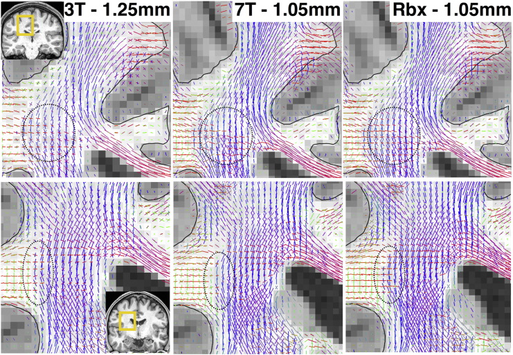
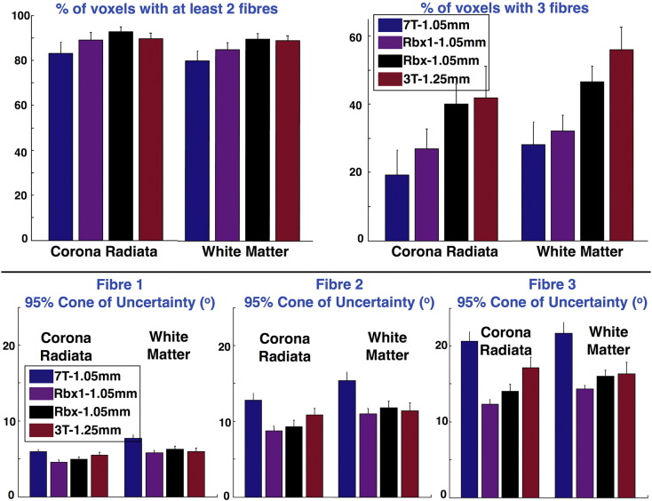
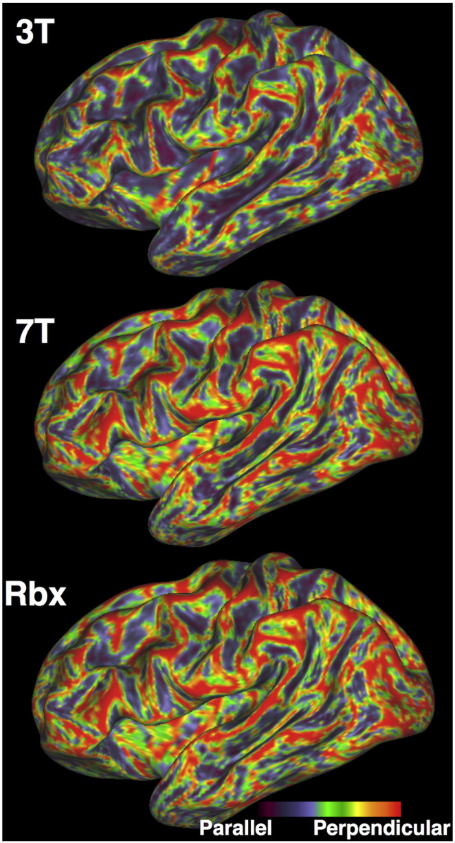
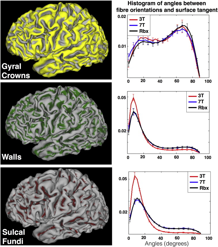
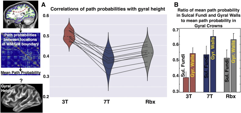
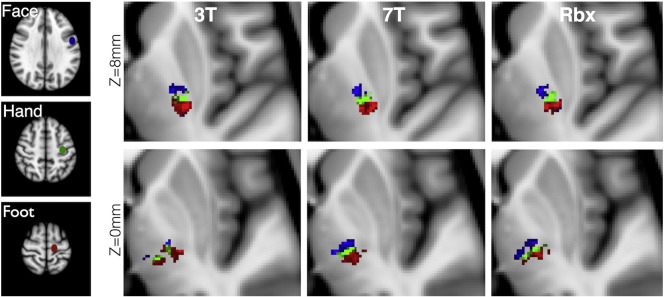
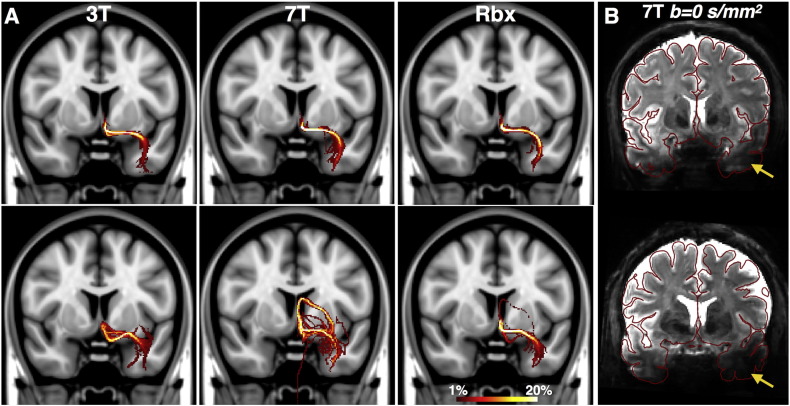
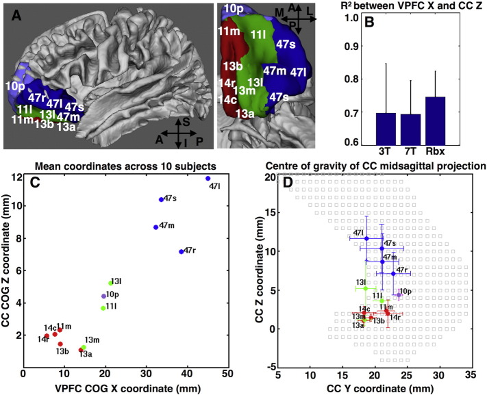
Determining the acquisition parameters in diffusion magnetic resonance imaging (dMRI) is governed by a series of trade-offs. Images of lower resolution have less spatial specificity but higher signal to noise ratio (SNR). At the same time higher angular contrast, important for resolving complex fibre patterns, also yields lower SNR. Considering these trade-offs, the Human Connectome Project (HCP) acquires high quality dMRI data for the same subjects at different field strengths (3T and 7T), which are publically released. Due to differences in the signal behavior and in the underlying scanner hardware, the HCP 3T and 7T data have complementary features in k- and q-space. The 3T dMRI has higher angular contrast and resolution, while the 7T dMRI has higher spatial resolution. Given the availability of these datasets, we explore the idea of fusing them together with the aim of combining their benefits. We extend a previously proposed data-fusion framework and apply it to integrate both datasets from the same subject into a single joint analysis. We use a generative model for performing parametric spherical deconvolution and estimate fibre orientations by simultaneously using data acquired under different protocols. We illustrate unique features from each dataset and how they are retained after fusion. We further show that this allows us to complement benefits and improve brain connectivity analysis compared to analyzing each of the datasets individually.
Overview
The claims and statistics of this paper haven’t been checked yet.
Run the check — free, no account needed. It reads the open-access text and checks the sources it cites.
Integrity signals
Registry
Cites
Statistics
Figures
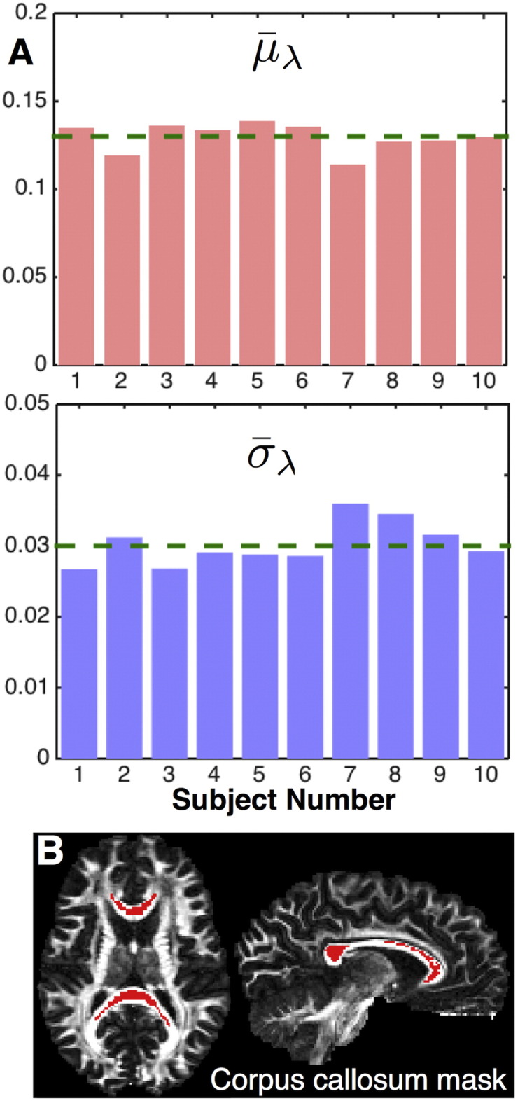
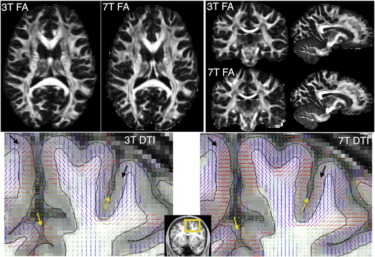
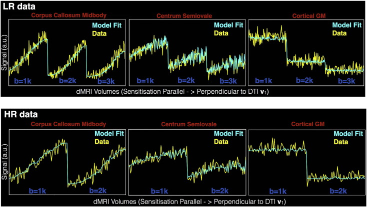
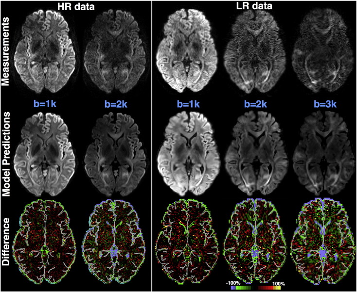
Verification
Claims the paper makes
The claims and statistics of this paper haven’t been checked yet.
Run the check — free, no account needed. It reads the open-access text and checks the sources it cites.
Claims other papers make about this one
Each is checked against this paper’s own text: does it say what the citing paper says it does?
The source backs part of the claim, not all of it — or backs it for a different population, condition or comparison.
In the citing paper
“Construction of the connectivity matrix has been described in several reviews (Sotiropoulos et al., 2016; Yeh et al., 2020) and includes two major steps. First, parcellation of the whole-brain tractogram is needed to compute all possible fiber pathways in the brain, i.e., white matter parcels connecting all pairs of gray matter regions (as described in Section 4.2). Then, a metric of “connectivity”
From Quantitative mapping of the brain’s structural connectivity using diffusion MRI tractography: A review (2022) · cites this paper as Sotiropoulos et al., 2016
Experimental — accuracy not yet measured
Self-check
Percentages, sums and reported differences re-computed from the paper’s own numbers.
The self-check needs the paper’s full text.
Citations
Cites
Fischl, B. (2012) · NeuroImage · doi:10.1016/j.neuroimage.2012.01.021 · Cited by 9,526
Spin Diffusion Measurements: Spin Echoes in the Presence of a Time-Dependent Field Gradient
Stejskal, E. O., & Tanner, J. E. (1965) · The Journal of Chemical Physics · doi:10.1063/1.1695690 · Cited by 8,239
The WU-Minn Human Connectome Project: An overview
Van Essen, D. C., Smith, S. M., Barch, D. M., Behrens, T. E. J., Yacoub, E., & Ugurbil, K. (2013) · NeuroImage · doi:10.1016/j.neuroimage.2013.05.041 · Cited by 5,651
Self-citationThe minimal preprocessing pipelines for the Human Connectome Project
Glasser, M. F., Sotiropoulos, S. N., Wilson, J. A., Coalson, T. S., Fischl, B., Andersson, J. L., Xu, J., Jbabdi, S., Webster, M., Polimeni, J. R., et al. (2013) · NeuroImage · doi:10.1016/j.neuroimage.2013.04.127 · Cited by 5,253
Self-citationDeep Brain Stimulation for Treatment-Resistant Depression
Mayberg, H. S., Lozano, A. M., Voon, V., McNeely, H. E., Seminowicz, D., Hamani, C., Schwalb, J. M., & Kennedy, S. H. (2005) · Neuron · doi:10.1016/j.neuron.2005.02.014 · Cited by 4,059
Accurate and robust brain image alignment using boundary-based registration
Greve, D. N., & Fischl, B. R. (2009) · NeuroImage · doi:10.1016/j.neuroimage.2009.06.060 · Cited by 3,553
Probabilistic diffusion tractography with multiple fibre orientations: What can we gain?
Behrens, T. E. J., Berg, H. J., Jbabdi, S., Rushworth, M. F. S., & Woolrich, M. W. (2007) · NeuroImage · doi:10.1016/j.neuroimage.2006.09.018 · Cited by 3,471
Self-citationAndersson, J. L. R., Skare, S., & Ashburner, J. (2003) · NeuroImage · doi:10.1016/s1053-8119(03)00336-7 · Cited by 3,469
Self-citationAndersson, J., & Sotiropoulos, S. N. (2015) · NeuroImage · doi:10.1016/j.neuroimage.2015.10.019 · Cited by 3,439
Self-citationNODDI: Practical in vivo neurite orientation dispersion and density imaging of the human brain
Zhang, H., Schneider, T., Wheeler-Kingshott, C. A., & Alexander, D. C. (2012) · NeuroImage · doi:10.1016/j.neuroimage.2012.03.072 · Cited by 3,288
Cited by
Sorted by citations
The Human Connectome Project's neuroimaging approach
Glasser, M. F., Smith, S. M., Marcus, D. S., Andersson, J. L. R., Auerbach, E. J., Behrens, T. E. J., Coalson, T. S., Harms, M. P., Jenkinson, M., Moeller, S., et al. (2016) · Nature Neuroscience · doi:10.1038/nn.4361 · Cited by 1,090
Self-citationImaging brain microstructure with diffusion MRI: practicality and applications
Alexander, D. C., Dyrby, T. B., Nilsson, M., & Zhang, H. G. (2017) · NMR in Biomedicine · doi:10.1002/nbm.3841 · Cited by 456
Hierarchical Heterogeneity across Human Cortex Shapes Large-Scale Neural Dynamics
Demirtaş, M., Burt, J. B., Helmer, M., Ji, J. L., Adkinson, B. D., Glasser, M. F., Essen, D. C. V., Sotiropoulos, S. N., Anticevic, A., & Murray, J. D. (2019) · Neuron · doi:10.1016/j.neuron.2019.01.017 · Cited by 343
Self-citationThe Human Connectome Project: A retrospective
Elam, J. S., Glasser, M. F., Harms, M. P., Sotiropoulos, S. N., Andersson, J., Burgess, G. C., Curtiss, S. W., Oostenveld, R., Larson‐Prior, L. J., Schoffelen, J., et al. (2021) · NeuroImage · doi:10.1016/j.neuroimage.2021.118543 · Cited by 340
Self-citationZhang, F., Daducci, A., He, Y., Schiavi, S., Seguin, C., Smith, R. E., Yeh, C.-H., Zhao, T., & O’Donnell, L. J. (2022) · NeuroImage · doi:10.1016/j.neuroimage.2021.118870 · Cited by 302
“Construction of the connectivity matrix has been described in several reviews [513, 423] and in-”
Building connectomes using diffusion MRI: why, how and but
Sotiropoulos, S. N., & Zalesky, A. (2019) · NMR in Biomedicine · doi:10.1002/nbm.3752 · Cited by 290
Self-citationHigh resolution whole brain diffusion imaging at 7 T for the Human Connectome Project
Vu, A. T., Auerbach, E. J., Lenglet, C., Moeller, S., Sotiropoulos, S. N., Jbabdi, S., Andersson, J., Yacoub, E. S., & Uǧurbil, K. (2015) · NeuroImage · doi:10.1016/j.neuroimage.2015.08.004 · Cited by 222
Self-citationJones, D. K., Alexander, D. C., Bowtell, R. W., Cercignani, M., Dell’Acqua, F., McHugh, D. J., Miller, K. L., Palombo, M., Parker, G. J. M., Rudrapatna, U. S., et al. (2018) · NeuroImage · doi:10.1016/j.neuroimage.2018.05.047 · Cited by 187
Imaging at ultrahigh magnetic fields: History, challenges, and solutions
Uǧurbil, K. (2017) · NeuroImage · doi:10.1016/j.neuroimage.2017.07.007 · Cited by 175
Automated processing pipeline for neonatal diffusion MRI in the developing Human Connectome Project
Bastiani, M., Andersson, J., Cordero‐Grande, L., Deprez, M., Hutter, J. M., Price, A. N., Makropoulos, A., Fitzgibbon, S. P., Hughes, E., Rueckert, D., et al. (2018) · NeuroImage · doi:10.1016/j.neuroimage.2018.05.064 · Cited by 173
Self-citationKarolak, A. M., Markov, D. A., McCawley, L. J., & Rejniak, K. A. (2018) · Journal of The Royal Society Interface · doi:10.1098/rsif.2017.0703 · Cited by 121
Automated hippocampal unfolding for morphometry and subfield segmentation with HippUnfold
DeKraker, J., Haast, R. A. M., Yousif, M. D., Karat, B. G., Lau, J. C., Köhler, S., & KHAN, A. R. (2022) · eLife · doi:10.7554/elife.77945 · Cited by 118
Abeysuriya, R., Hadida, J., Sotiropoulos, S. N., Jbabdi, S., Becker, R., Hunt, B. A. E., Brookes, M. J., & Woolrich, M. W. (2018) · PLoS Computational Biology · doi:10.1371/journal.pcbi.1006007 · Cited by 96
Self-citationNext-generation neural mass and field modeling
Byrne, Á., O’Dea, R. D., Forrester, M., Ross, J., & Coombes, S. (2019) · Journal of Neurophysiology · doi:10.1152/jn.00406.2019 · Cited by 101
Time‐efficient and flexible design of optimized multishell HARDI diffusion
Hutter, J. M., Tournier, J., Price, A. N., Cordero‐Grande, L., Hughes, E., Malik, S., Steinweg, J. K., Bastiani, M., Sotiropoulos, S. N., Jbabdi, S., et al. (2017) · Magnetic Resonance in Medicine · doi:10.1002/mrm.26765 · Cited by 93
Self-citationAutio, J. A., Glasser, M. F., Ose, T., Donahue, C. J., Bastiani, M., Ohno, M., Kawabata, Y., Urushibata, Y., Murata, K., Nishigori, K., et al. (2020) · NeuroImage · doi:10.1016/j.neuroimage.2020.116800 · Cited by 91
Self-citationOccipital White Matter Tracts in Human and Macaque
Takemura, H., Pestilli, F., Weiner, K. S., Keliris, G. A., Landi, S. M., Sliwa, J., Ye, F. Q., Barnett, M., Leopold, D. A., Freiwald, W. A., et al. (2017) · Cerebral Cortex · doi:10.1093/cercor/bhx070 · Cited by 87
Clinical vascular imaging in the brain at 7 T
Cocker, L. J. L. D., Lindenholz, A., Zwanenburg, J. J. M., van der Kolk, A. G., Zwartbol, M. H. T., Luijten, P. R., & Hendrikse, J. (2016) · NeuroImage · doi:10.1016/j.neuroimage.2016.11.044 · Cited by 81
Tewarie, P. K. B., Abeysuriya, R., Byrne, Á., O’Neill, G. C., Sotiropoulos, S. N., Brookes, M. J., & Coombes, S. (2018) · NeuroImage · doi:10.1016/j.neuroimage.2018.10.079 · Cited by 76
Self-citationAydogan, D. B., Jacobs, R., Dulawa, S., Thompson, S. L., Francois, M. C., Toga, A. W., Dong, H., Knowles, J. A., & Shi, Y. (2018) · Brain Structure and Function · doi:10.1007/s00429-018-1663-8 · Cited by 72
Koike, S., Tanaka, S., Okada, T., Aso, T., Yamashita, A., Yamashita, O., Asano, M., Maikusa, N., Morita, K., Okada, N., et al. (2021) · NeuroImage Clinical · doi:10.1016/j.nicl.2021.102600 · Cited by 65
Within brain area tractography suggests local modularity using high resolution connectomics
Taylor, P. N., Wang, Y., & Kaiser, M. (2017) · Scientific Reports · doi:10.1038/srep39859 · Cited by 67
Uǧurbil, K. (2016) · Philosophical Transactions of the Royal Society B Biological Sciences · doi:10.1098/rstb.2015.0361 · Cited by 68
High‐resolution whole‐brain diffusion MRI at 7T using radiofrequency parallel transmission
Wu, X., Auerbach, E. J., Vu, A. T., Moeller, S., Lenglet, C., Schmitter, S., de Moortele, P. V., Yacoub, E. S., & Uǧurbil, K. (2018) · Magnetic Resonance in Medicine · doi:10.1002/mrm.27189 · Cited by 62
Self-citationWarrington, S., Thompson, E., Bastiani, M., Dubois, J., Baxter, L., Slater, R., Jbabdi, S., Mars, R. B., & Sotiropoulos, S. N. (2022) · Science Advances · doi:10.1126/sciadv.abq2022 · Cited by 57
Self-citationFan, Q., Eichner, C., Afzali, M., Mueller, L., Tax, C. M. W., Davids, M., Mahmutović, M., Keil, B. R., Bilgiç, B., Setsompop, K., et al. (2022) · NeuroImage · doi:10.1016/j.neuroimage.2022.118958 · Cited by 54
Diffusion MRI of the human brain at ultra-high field (UHF): A review
Gallichan, D. (2017) · NeuroImage · doi:10.1016/j.neuroimage.2017.04.037 · Cited by 44
Mitigating gyral bias in cortical tractography via asymmetric fiber orientation distributions
Wu, Y., Hong, Y., Feng, Y., Shen, D. G., & Yap, P. (2019) · Medical Image Analysis · doi:10.1016/j.media.2019.101543 · Cited by 43
A causal role for the pulvinar in coordinating task‐independent cortico–cortical interactions
Eradath, M. K., Pinsk, M. A., & Kästner, S. (2021) · The Journal of Comparative Neurology · doi:10.1002/cne.25193 · Cited by 45
Multicenter dataset of multi-shell diffusion MRI in healthy traveling adults with identical settings
Tong, Q., He, H., Gong, T., Li, C., Liang, P., Qian, T., Sun, Y., Ding, Q., Li, K., & Zhong, J. (2020) · Scientific Data · doi:10.1038/s41597-020-0493-8 · Cited by 43
Improvement of magnetic resonance imaging using a wireless radiofrequency resonator array
Alipour, A., Seifert, A. C., Delman, B. N., Robson, P. M., Shrivastava, R. K., Hof, P. R., Adriany, G., Fayad, Z. A., & Balchandani, P. (2021) · Scientific Reports · doi:10.1038/s41598-021-02533-3 · Cited by 40
Cortical fibers orientation mapping using in-vivo whole brain 7 T diffusion MRI
Gülban, Ö. F., Martino, F. D., Vu, A. T., Yacoub, E. S., Uǧurbil, K., & Lenglet, C. (2018) · NeuroImage · doi:10.1016/j.neuroimage.2018.05.010 · Cited by 39
Self-citationTan, X., Zhou, Z., Gao, J. J., Meng, F., Yu, Y., Zhang, J., He, F., Wei, R., Wang, J., Peng, G., et al. (2019) · NeuroImage Clinical · doi:10.1016/j.nicl.2019.101702 · Cited by 40
Ma, X., Uǧurbil, K., & Wu, X. (2020) · NeuroImage · doi:10.1016/j.neuroimage.2020.116852 · Cited by 40
The role of node dynamics in shaping emergent functional connectivity patterns in the brain
Forrester, M., Crofts, J. J., Sotiropoulos, S. N., Coombes, S., & O’Dea, R. D. (2020) · Network Neuroscience · doi:10.1162/netn_a_00130 · Cited by 34
Self-citationModelling white matter in gyral blades as a continuous vector field
Cottaar, M., Bastiani, M., Boddu, N., Glasser, M. F., Haber, S. N., Essen, D. C. V., Sotiropoulos, S. N., & Jbabdi, S. (2020) · NeuroImage · doi:10.1016/j.neuroimage.2020.117693 · Cited by 36
Self-citationHIgh b-value and high Resolution Integrated Diffusion (HIBRID) imaging
Fan, Q., Nummenmaa, A. R., Polimeni, J. R., Witzel, T., Huang, S. Y., Wedeen, V. J., Rosen, B. R., & Wald, L. L. (2017) · NeuroImage · doi:10.1016/j.neuroimage.2017.02.002 · Cited by 34
Wu, X., Auerbach, E. J., Vu, A. T., Moeller, S., de Moortele, P. V., Yacoub, E. S., & Uǧurbil, K. (2018) · NeuroImage · doi:10.1016/j.neuroimage.2018.09.038 · Cited by 31
Self-citationHarmonizing Diffusion MRI Data Across Magnetic Field Strengths
Karayumak, S. C., Kubicki, M. R., & Yogesh Rathi, A. (2018) · Lecture notes in computer science · doi:10.1007/978-3-030-00931-1_14 · Cited by 28
Joint modelling of diffusion MRI and microscopy
Howard, A. F. D., Mollink, J., Kleinnijenhuis, M., Pallebage‐Gamarallage, M. M., Bastiani, M., Cottaar, M., Miller, K. L., & Jbabdi, S. (2019) · NeuroImage · doi:10.1016/j.neuroimage.2019.116014 · Cited by 29
Self-citationDiffusion Acceleration with Gaussian process Estimated Reconstruction (DAGER)
Wu, W., Koopmans, P. J., Andersson, J., & Miller, K. L. (2019) · Magnetic Resonance in Medicine · doi:10.1002/mrm.27699 · Cited by 27
Self-citationDiffusion Imaging in the Post HCP Era
Moeller, S., Pisharady, P. K., Andersson, J., Akçakaya, M., Harel, N., Ma, R. E., Wu, X., Yacoub, E. S., Lenglet, C., & Uǧurbil, K. (2020) · Journal of Magnetic Resonance Imaging · doi:10.1002/jmri.27247 · Cited by 30
Self-citationBranzoli, F., Ercan, E., Valabrègue, R., Wood, E. T., Buijs, M., WEBB, A. G., & Ronen, I. (2016) · Neurobiology of Aging · doi:10.1016/j.neurobiolaging.2016.07.022 · Cited by 29
Post-Concussive Vestibular Dysfunction Is Related to Injury to the Inferior Vestibular Nerve
Gard, A., Al-Husseini, A., Kornaropoulos, E., Maio, A. D., Tegner, Y., Björkman‐Burtscher, I. M., Bloch, K. M., Nilsson, M., Magnusson, M., & Marklund, N. (2022) · Journal of Neurotrauma · doi:10.1089/neu.2021.0447 · Cited by 29
Ma, R. E., Akçakaya, M., Moeller, S., Auerbach, E. J., Uǧurbil, K., & de Moortele, P. V. (2020) · NeuroImage · doi:10.1016/j.neuroimage.2020.116861 · Cited by 24
Self-citationAccuracy and reliability of diffusion imaging models
Seider, N. A., Adeyemo, B., Miller, R. L., Newbold, D. J., Hampton, J. M., Scheidter, K. M., Rutlin, J. R., Laumann, T. O., Roland, J. L., Montez, D. F., et al. (2022) · NeuroImage · doi:10.1016/j.neuroimage.2022.119138 · Cited by 28
Rationalization of using the MR diffusion imaging in B12 deficiency
Kanat, A., Polat, H. B., Çeliker, F. B., Tüfekçi, A., Beyazal, M., Ardic, G., & Turan, A. (2020) · Annals of Indian Academy of Neurology · doi:10.4103/aian.aian_485_18 · Cited by 24
Kim, H., Baek, A., Choi, G., Lee, J., Yang, J.-U., Jung, H., Lee, T., Kim, D. K., Kim, M., Cho, A. E., et al. (2020) · Biomaterials · doi:10.1016/j.biomaterials.2020.119939 · Cited by 23
Voineskos, A. N., Blumberger, D. M., Schifani, C., Hawco, C. S., Dickie, E. W., Rajji, T. K., Mulsant, B. H., Foussias, G., Wang, W., & Daskalakis, Z. J. (2020) · Biological Psychiatry Cognitive Neuroscience and Neuroimaging · doi:10.1016/j.bpsc.2020.11.011 · Cited by 21
Structural connectivity-based segmentation of the human entorhinal cortex
Syversen, I. F., Witter, M. P., Kobro‐Flatmoen, A., Goa, P. E., Schröder, T. N., & Doeller, C. F. (2021) · NeuroImage · doi:10.1016/j.neuroimage.2021.118723 · Cited by 22
Ultra-high field (10.5T) diffusion-weighted MRI of the macaque brain
Grier, M. D., Yacoub, E. S., Adriany, G., Lagore, R., Harel, N., Zhang, R., Lenglet, C., Uǧurbil, K., Zimmermann, J., & Heilbronner, S. R. (2022) · NeuroImage · doi:10.1016/j.neuroimage.2022.119200 · Cited by 19
Self-citationPascual‐Diaz, S., Varriano, F., Pineda, J., & Prats‐Galino, A. (2020) · NeuroImage · doi:10.1016/j.neuroimage.2020.117260 · Cited by 18
Baxter, L., Moultrie, F., Fitzgibbon, S. P., Aspbury, M., Mansfield, R. C., Bastiani, M., Rogers, R., Jbabdi, S., Duff, E. P., & Slater, R. (2021) · Nature Communications · doi:10.1038/s41467-021-22960-0 · Cited by 22
Self-citationSepehrband, F., O’Brien, K., & Barth, M. (2017) · Magnetic Resonance in Medicine · doi:10.1002/mrm.26608 · Cited by 16
Non-negative data-driven mapping of structural connections with application to the neonatal brain
Thompson, E., Mohammadi‐Nejad, A., Robinson, E. C., Andersson, J., Jbabdi, S., Glasser, M. F., Bastiani, M., & Sotiropoulos, S. N. (2020) · NeuroImage · doi:10.1016/j.neuroimage.2020.117273 · Cited by 16
Self-citationLaterality and Sex Differences of Human Lateral Habenula Afferent and Efferent Fiber Tracts
Hitti, F. L., Parker, D., Yang, A. I., Brem, S. S., & Verma, R. (2022) · Frontiers in Neuroscience · doi:10.3389/fnins.2022.837624 · Cited by 14
Quinones, J. F., Pavan, T., Liu, X., Thiel, C. M., Heep, A., & Hildebrandt, A. (2022) · NeuroImage · doi:10.1016/j.neuroimage.2022.119141 · Cited by 9
Kornaropoulos, E., Winzeck, S., Rumetshofer, T., Wikstrom, A., Knutsson, L., Correia, M., Sundgren, P. C., & Nilsson, M. (2022) · Frontiers in Neurology · doi:10.3389/fneur.2022.837385 · Cited by 11
Forrester, M., Petros, S., Cattell, O., Lai, Y. M., O’Dea, R. D., Sotiropoulos, S. N., & Coombes, S. (2024) · PLoS Computational Biology · doi:10.1371/journal.pcbi.1012647 · Cited by 10
Self-citationSuder, P. M., Xu, J., & Dunson, D. B. (2025) · Statistical Science · doi:10.1214/25-sts987 · Cited by 28
Pisharady, P. K., Sotiropoulos, S. N., Duarte‐Carvajalino, J. M., Sapiro, G., & Lenglet, C. (2017) · NeuroImage · doi:10.1016/j.neuroimage.2017.06.052 · Cited by 10
Self-citationPatriat, R., Palnitkar, T., Chandrasekaran, J., Wong, K. S., Braun, H. C., Yacoub, E. S., McGovern, R. A., Aman, J. E., Cooper, S. E., Vitek, J. L., et al. (2024) · Frontiers in Human Neuroscience · doi:10.3389/fnhum.2024.1324710 · Cited by 9
Self-citationVerschuur, A. S., King, R., Tax, C. M. W., Boomsma, M. F., van Wezel‐Meijler, G., Leemans, A., & Leijser, L. M. (2024) · Pediatric Research · doi:10.1038/s41390-024-03463-2 · Cited by 9
DIMOND: DIffusion Model OptimizatioN with Deep Learning
Li, Z., Li, Z., Bilgiç, B., Lee, H., Ying, K., Huang, S. Y., Liao, H., & Tian, Q. (2024) · Advanced Science · doi:10.1002/advs.202307965 · Cited by 9
When Diffusion MRI Meets Diffusion Model: A Novel Deep Generative Model for Diffusion MRI Generation
Zhu, X., Zhang, W., Li, Y., O’Donnell, L. J., & Zhang, F. (2024) · Lecture notes in computer science · doi:10.1007/978-3-031-72069-7_50 · Cited by 8
Cross-species neuroanatomy in primates using tractography
Sotiropoulos, S. N., de Schotten, M. T., Haber, S. N., & Forkel, S. J. (2025) · Brain Structure and Function · doi:10.1007/s00429-025-02914-8 · Cited by 6
Self-citationLützkendorf, R., Heidemann, R. M., Feiweier, T., Luchtmann, M., Baecke, S., Kaufmann, J., Stadler, J., Budinger, E., & Bernarding, J. (2018) · Magnetic Resonance Materials in Physics Biology and Medicine · doi:10.1007/s10334-018-0705-9 · Cited by 6
T r G A N e t : Transforming 3T to 7T dMRI using Trapezoidal Rule and Graph based Attention Modules
Jha, R. R., Kumar, B., Pathak, S., Bhavsar, A. V., & Nigam, A. (2023) · Medical Image Analysis · doi:10.1016/j.media.2023.102806 · Cited by 6
Howell, A. M., Warrington, S., Fonteneau, C., Cho, Y., Sotiropoulos, S. N., Murray, J. D., & Anticevic, A. (2024) · eLife · doi:10.7554/elife.95018 · Cited by 5
Self-citationIn Vivo Quantification of White Matter Pathways in the Human Hippocampus
Gumus, M., Bourganos, A., & Mack, M. L. (2025) · Human Brain Mapping · doi:10.1002/hbm.70417 · Cited by 4
White Matter Connectivity between Structures of the Basal Ganglia using 3T and 7T
Shim, J., & Baek, H. (2021) · Neuroscience · doi:10.1016/j.neuroscience.2021.12.034 · Cited by 4
Schmid, A. B., Ridgway, L., Hailey, L. H., Tachrount, M., Probert, F., Martin, K. R., Scott, W., Crombez, G., Price, C., Robinson, C., et al. (2023) · BMJ Open · doi:10.1136/bmjopen-2023-072832 · Cited by 6
A gradient of hemisphere-specific dorsal to ventral processing routes in parieto-premotor networks
Jüchtern, M., Shaikh, U. J., Caspers, S., & Binkofski, F. (2024) · Network Neuroscience · doi:10.1162/netn_a_00407 · Cited by 4
Syversen, I. F., Reznik, D., Witter, M. P., Kobro‐Flatmoen, A., Schröder, T. N., & Doeller, C. F. (2024) · Hippocampus · doi:10.1002/hipo.23639 · Cited by 5
Girard, G., Aydogan, D. B., Dell’Acqua, F., Leemans, A., Descoteaux, M., & Sotiropoulos, S. N. (2025) · Elsevier eBooks · doi:10.1016/b978-0-12-818894-1.00030-6 · Cited by 4
Self-citationWu, Y., Hong, Y., Ahmad, S., & Yap, P. (2021) · Lecture notes in computer science · doi:10.1007/978-3-030-87234-2_44 · Cited by 4
Pascual‐Diaz, S., Pineda, J., Serra, L., Varriano, F., & Prats‐Galino, A. (2019) · PLoS ONE · doi:10.1371/journal.pone.0224598 · Cited by 3
Im, S.-J., Lee, J., & Kim, S. (2021) · Experimental Neurobiology · doi:10.5607/en20056 · Cited by 3
Caron, A. V., Shmuel, A., Hao, Z., & Descoteaux, M. (2023) · Frontiers in Neuroinformatics · doi:10.3389/fninf.2023.1191200 · Cited by 3
Carnevale, L., & Lembo, G. (2024) · Cardiovascular Research · doi:10.1093/cvr/cvae165 · Cited by 3
Koike, S., Tanaka, S. C., Okada, T., Aso, T., Asano, M., Maikusa, N., Morita, K., Okada, N., Fukunaga, M., Uematsu, A., et al. (2020) · bioRxiv (Cold Spring Harbor Laboratory) · doi:10.1101/2020.05.05.076273 · Cited by 3
Howell, A. M., Warrington, S., Fonteneau, C., Cho, Y., Sotiropoulos, S. N., Murray, J. D., & Anticevic, A. (2023) · bioRxiv (Cold Spring Harbor Laboratory) · doi:10.1101/2023.07.22.550168 · Cited by 4
Self-citationDiffusion Measures of Subcortical Structures Using High-Field MRI
Baek, H. (2023) · Brain Sciences · doi:10.3390/brainsci13030391 · Cited by 2
Radetz, A., & Groppa, S. (2021) · Neuromethods · doi:10.1007/978-1-0716-1213-2_3 · Cited by 2
Precision Diffusion ImagingPreprint
Seider, N. A., Adeyemo, B., Miller, R. L., Newbold, D. J., Hampton, J. M., Scheidter, K. M., Rutlin, J. R., Laumann, T. O., Roland, J. L., Montez, D. F., et al. (2021) · bioRxiv (Cold Spring Harbor Laboratory) · doi:10.1101/2021.02.19.432023 · Cited by 2
Syversen, I. F., Reznik, D., Witter, M. P., Kobro‐Flatmoen, A., Schröder, T. N., & Doeller, C. F. (2022) · bioRxiv (Cold Spring Harbor Laboratory) · doi:10.1101/2022.12.23.520976 · Cited by 2
Personalized circuit modeling captures variation in cortical functional connectivityPreprint
Cooper, R. A., Demirtaş, M., Burt, J. B., Howell, A. M., Ji, J., Repovš, G., Sotiropoulos, S. N., Anticevic, A., & Murray, J. D. (2024) · bioRxiv (Cold Spring Harbor Laboratory) · doi:10.1101/2024.02.19.581085 · Cited by 2
Self-citationTaskin, E., Girard, G., Haro, J. L. V., Rafael‐Patiño, J., Garyfallidis, E., Thiran, J., & Canales-Rodríguez, E. J. (2025) · NeuroImage · doi:10.1016/j.neuroimage.2025.121656 · Cited by 1
Diffusion MRI acquisition for tractography: Diffusion sequences
Campbell, J. S. W., Baete, S. H., Cohen‐Adad, J., Tournier, J., Szczepankiewicz, F., Beaulieu, C., Baron, C. A., Mani, M., Setsompop, K., Liao, C., et al. (2025) · Elsevier eBooks · doi:10.1016/b978-0-12-818894-1.00019-7 · Cited by 1
Davis, A. D., Hassel, S., Arnott, S. R., Hall, G. B., Harris, J. K., Zamyadi, M., Downar, J. H., Frey, B. N., Lam, R. W. M., Kennedy, S. H., et al. (2021) · Physics in Medicine and Biology · doi:10.1088/1361-6560/ac46de · Cited by 2
Howell, A. M., Warrington, S., Fonteneau, C., Cho, Y., Sotiropoulos, S. N., Murray, J. D., & Anticevic, A. (2024) · eLife · doi:10.7554/elife.95018.1 · Cited by 1
Self-citationDrawing the boundaries of expertise: Who is a mathematician?
Popescu, T., & Kadosh, R. C. (2019) · Cortex · doi:10.1016/j.cortex.2019.04.020
Caron, A. V., Shmuel, A., Hao, Z., & Descoteaux, M. (2021) · bioRxiv (Cold Spring Harbor Laboratory) · doi:10.1101/2021.11.22.469616
Technology for Ultrahigh Field Imaging
Uǧurbil, K. (2022) · Wiley eBooks · doi:10.1002/9783527827244.ch4
Shi, L., Woodward, A., & Igarashi, J. (2022) · bioRxiv (Cold Spring Harbor Laboratory) · doi:10.1101/2022.12.25.521904
Shirazinodeh, A., Faraji, H., Javidi, S. S., Jafari, A. H., Nazem-Zadeh, M.-R., & Rad, H. S. (2023) · Journal of Biomedical Physics and Engineering · doi:10.31661/jbpe.v0i0.2108-1387
An Image Quality Transfer Technique for Localising Deep Brain Stimulation TargetsPreprint
Zheng, Y., Akram, H., Li, Z., Smith, S. M., & Jbabdi, S. (2024) · bioRxiv (Cold Spring Harbor Laboratory) · doi:10.1101/2024.03.18.584979
Self-citationVoxel-Wise Fusion of 3T and 7T Diffusion MRI Data to Extract more Accurate Fiber Orientations
Wu, Z., Weng, X., Shen, J. F., & Hong, M. (2024) · Brain Topography · doi:10.1007/s10548-024-01046-2
Huang, Z., Charalambous, C. C., Chen, M., Kim, T., Sokhadze, E. M., Song, A. W., Jung, S., Shekhar, S., Feld, J., Jiang, X., et al. (2024) · medRxiv · doi:10.1101/2024.09.12.24313472
Brain local structural connectomes and the subtypes of the medial temporal lobe parcellationsPreprint
Li, Z., Ma, J., Bai, H., Deng, B., Lin, J., & Wang, W. (2024) · Research Square · doi:10.21203/rs.3.rs-4893321/v1
Metadata
- Authors
- Sotiropoulos, S. N., Hernández-Fernández, M., Vu, A. T., Andersson, J. L., Moeller, S., Yacoub, E., Lenglet, C., Ugurbil, K., Behrens, T. E. J., & Jbabdi, S.
- Affiliations
- University of Oxford (GB)
- University of Minnesota (US)
- Wellcome Centre for Human Neuroimaging (GB)
- Corresponding author
- Sotiropoulos, Stamatios N.
- ORCID
- Venue
- NeuroImage
- Publisher
- Elsevier BV
- Published
- 2016-07
- Volume
- 134
- Pages
- 396-409
- ISSN
- 1053-8119 (ISSN-L)
- PMC
- PMC6318224
- OpenAlex
- W2328941635
- Cited by
- 110
- References
- 57
- Citations by year
- 2026: 2 · 2025: 14 · 2024: 15 · 2023: 6 · 2022: 13 · 2021: 13 · 2020: 13 · 2019: 8 · 2018: 11 · 2017: 10 · 2016: 4
- FWCI
- 9.55
- Type
- journal article
- Language
- en
- Open access
- hybrid
- doi.org
- Locations
- NeuroImage (publishedVersion, cc-by)
- Europe PMC (PubMed Central) (publishedVersion, cc-by)
- PubMed Central (publishedVersion, cc-by)
- PubMed (publishedVersion)
- Repository@Nottingham (University of Nottingham) (submittedVersion, cc-by)
- Funders
- Human Connectome Project (1U54MH091657-01)
- NIH (P41 EB015894)
- UK EPSRC (EP/L023067/1)
- UK MRC (MR/L009013/1)
- Topics
- Health Sciences › Medicine › Radiology, Nuclear Medicine and Imaging › Advanced Neuroimaging Techniques and Applications
- Life Sciences › Neuroscience › Cognitive Neuroscience › Functional Brain Connectivity Studies
- Health Sciences › Medicine › Radiology, Nuclear Medicine and Imaging › Advanced MRI Techniques and Applications
- Keywords
- diffusion MRI, data fusion, Human Connectome Project, brain connectivity, generative models, high-field MRI
- MeSH terms
- Adult, Algorithms, Brain, Female, Humans, Image Enhancement, Image Interpretation, Computer-Assisted, Male, Sensitivity and Specificity, Subtraction Technique, Reproducibility of Results, Diffusion Tensor Imaging, Connectome, White Matter
About these checks
Registry, retraction, Cites and statistics results are computed, not judged, with one exception: a printed reference that no index lists is read once by a model before it counts as a citation error. Claims are extracted by a model and kept only when their quote appears verbatim in the text; each cited source is then checked, with a model’s help, for whether it says what the claim relies on. Those verdicts can be wrong — read the claim’s quote and the cited source before relying on one.
Statistics and arithmetic are recomputed, not judged.
Confidence bands are shown only for fields calibrated on our annotated test set. None is calibrated yet, so no band is shown.
What counts as a claim ›How we measure confidence ›How we check this ›
Are you an author, or do you see a problem with this page? Request a review
