

The DOI matches its Crossref record; 79 of the 79 references it cites were found in a registry or an index.
Unraveling the secrets of white matter--bridging the gap between cellular, animal and human imaging studies
Open accessAbstract
The CNS white matter makes up about half of the human brain, and with advances in human imaging it is increasingly becoming clear that changes in the white matter play a major role in shaping human behavior and learning. However, the mechanisms underlying these white matter changes remain poorly understood. Within this special issue of Neuroscience on white matter, recent advances in our knowledge of the function of white matter, from the molecular level to human imaging, are reviewed. Collaboration between fields is essential to understand the function of the white matter, but due to differences in methods and field-specific 'language', communication is often hindered. In this review, we try to address this hindrance by introducing the methods and providing a basic background to myelin biology and human imaging as a prelude to the other reviews within this special issue.
Overview
The claims and statistics of this paper haven’t been checked yet.
Run the check — free, no account needed. It reads the open-access text and checks the sources it cites.
Integrity signals
Registry
Cites
Statistics
Figures
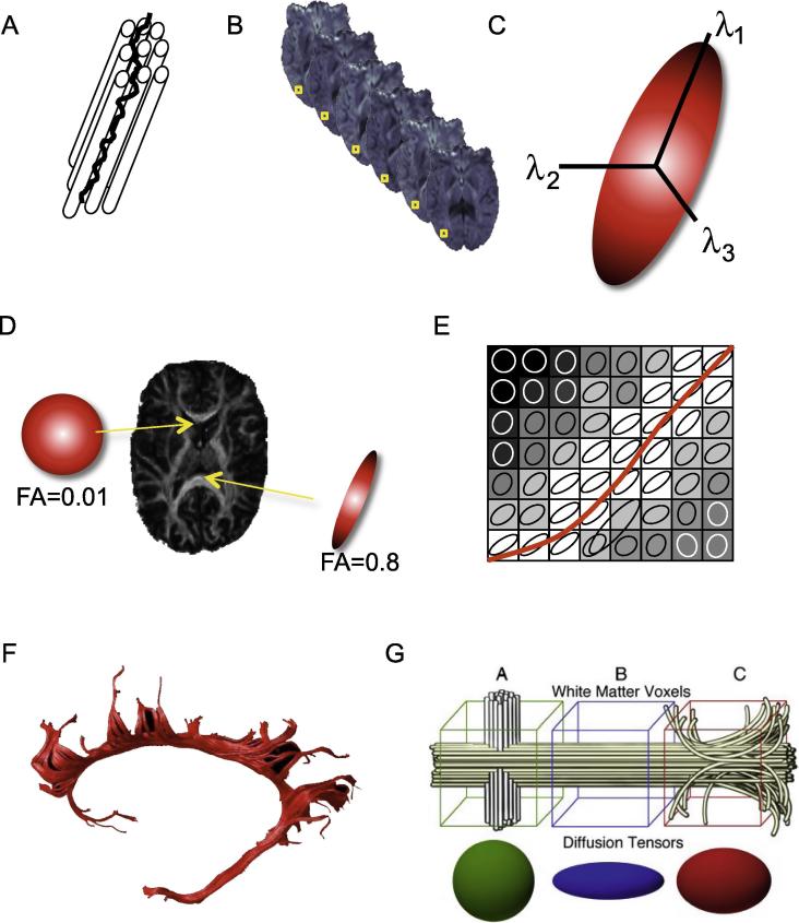
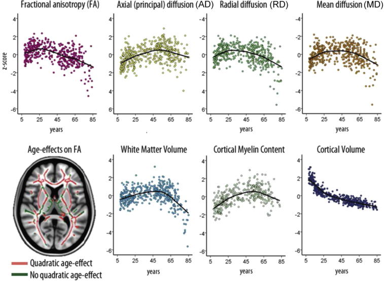
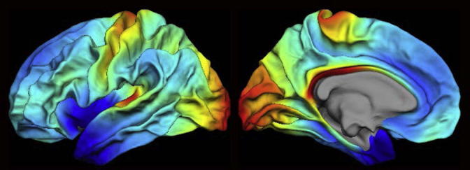
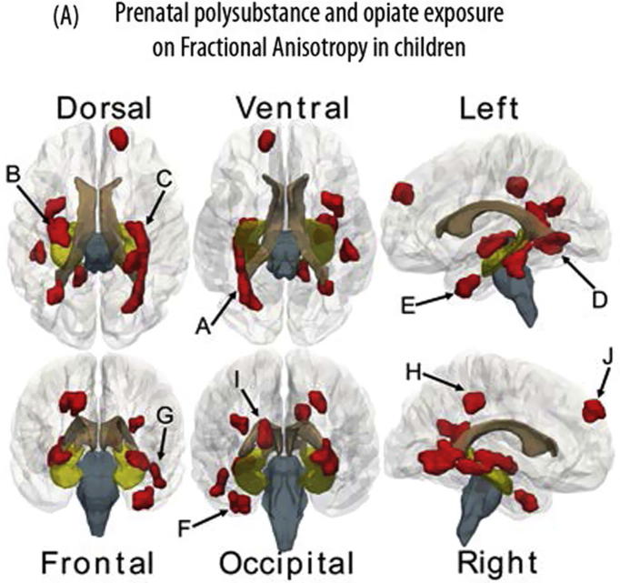
Verification
Claims the paper makes
The claims and statistics of this paper haven’t been checked yet.
Run the check — free, no account needed. It reads the open-access text and checks the sources it cites.
Claims other papers make about this one
Each is checked against this paper’s own text: does it say what the citing paper says it does?
The source backs part of the claim, not all of it — or backs it for a different population, condition or comparison.
In the citing paper
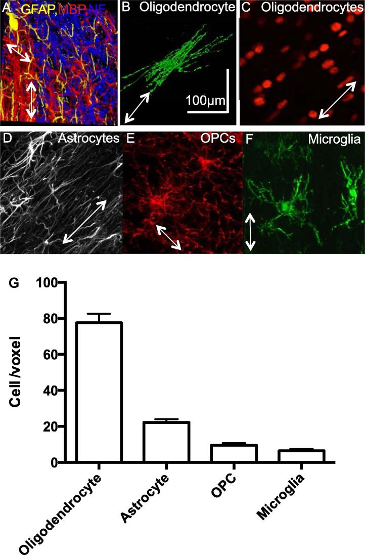
“However, even at this 100 μm resolution and ∼17 h scan times, each imaging voxel can contain anywhere from 1,000 to 13,000 axons, over 80 oligodendrocytes, and more than 20 astrocytes (Walhovd et al., 2014).”
From The role of myelination in measures of white matter integrity: Combination of diffusion tensor imaging and two-photon microscopy of CLARITY intact brains (2017) · cites this paper as Walhovd et al., 2014
Experimental — accuracy not yet measured
Self-check
Percentages, sums and reported differences re-computed from the paper’s own numbers.
The self-check needs the paper’s full text.
Citations
Cites
Fischl, B., Salat, D. H., Busa, E., Albert, M., Dieterich, M., Haselgrove, C., van der Kouwe, A., Killiany, R., Kennedy, D., Klaveness, S., et al. (2002) · Neuron · doi:10.1016/s0896-6273(02)00569-x · Cited by 8,610
Le Bihan, D., Breton, E., Lallemand, D., Grenier, P., Cabanis, E., & Laval-Jeantet, M. (1986) · Radiology · doi:10.1148/radiology.161.2.3763909 · Cited by 3,912
Estimation of the Effective Self-Diffusion Tensor from the NMR Spin Echo
Basser, P. J., Mattiello, J., & Bihan, D. L. (1994) · Journal of Magnetic Resonance Series B · doi:10.1006/jmrb.1994.1037 · Cited by 3,656
Probabilistic diffusion tractography with multiple fibre orientations: What can we gain?
Behrens, T. E. J., Berg, H. J., Jbabdi, S., Rushworth, M. F. S., & Woolrich, M. W. (2007) · NeuroImage · doi:10.1016/j.neuroimage.2006.09.018 · Cited by 3,471
Self-citationWithin-subject template estimation for unbiased longitudinal image analysis
Reuter, M., Schmansky, N. J., Rosas, H. D., & Fischl, B. (2012) · NeuroImage · doi:10.1016/j.neuroimage.2012.02.084 · Cited by 2,356
Song, S.-K., Sun, S.-W., Ju, W.-K., Lin, S.-J., Cross, A. H., & Neufeld, A. H. (2003) · NeuroImage · doi:10.1016/j.neuroimage.2003.07.005 · Cited by 1,738
Plasticity in gray and white: neuroimaging changes in brain structure during learning
Zatorre, R. J., Fields, R. D., & Johansen-Berg, H. (2012) · Nature Neuroscience · doi:10.1038/nn.3045 · Cited by 1,685
Self-citationTraining induces changes in white-matter architecture
Scholz, J., Klein, M. C., Behrens, T. E. J., & Johansen-Berg, H. (2009) · Nature Neuroscience · doi:10.1038/nn.2412 · Cited by 1,508
Self-citationUniquely Hominid Features of Adult Human Astrocytes
Oberheim, N. A., Takano, T., Han, X., He, W., Lin, J. H. C., Wang, F., Xu, Q., Wyatt, J. D., Pilcher, W., Ojemann, J. G., et al. (2009) · The Journal of Neuroscience · doi:10.1523/jneurosci.4707-08.2009 · Cited by 1,488
Neuronal activity promotes oligodendrogenesis and adaptive myelination in the mammalian brain
Gibson, E. M., Purger, D., Mount, C. W., Goldstein, A. K., Lin, G. L., Wood, L. S., Inema, I., Miller, S. E., Bieri, G., Zuchero, J. B., et al. (2014) · Science · doi:10.1126/science.1252304 · Cited by 1,472
Cited by
Sorted by citations
Verkhratsky, A., & Nedergaard, M. (2018) · Physiological Reviews · doi:10.1152/physrev.00042.2016 · Cited by 1,678
White matter and cognition: making the connection
Filley, C. M., & Fields, R. D. (2016) · Journal of Neurophysiology · doi:10.1152/jn.00221.2016 · Cited by 479
Astrocytes in physiological aging and Alzheimer’s disease
Rodríguez-Arellano, J. J., Parpura, V., Zorec, R., & Verkhratsky, A. (2016) · Neuroscience · doi:10.1016/j.neuroscience.2015.01.007 · Cited by 439
White Matter Plasticity in the Adult Brain
Sampaio‐Baptista, C., & Johansen‐Berg, H. (2017) · Neuron · doi:10.1016/j.neuron.2017.11.026 · Cited by 432
Self-citationSexton, C. E., Betts, J. F., Demnitz, N., Dawes, H., Ebmeier, K. P., & Johansen‐Berg, H. (2015) · NeuroImage · doi:10.1016/j.neuroimage.2015.09.071 · Cited by 278
Self-citationBrain structure and cognitive ability in healthy aging: a review on longitudinal correlated change
Oschwald, J., Guye, S., Liem, F., Rast, P., Willis, S. L., Röcke, C., Jäncke, L., Martin, M., & Mérillat, S. (2019) · Reviews in the Neurosciences · doi:10.1515/revneuro-2018-0096 · Cited by 273
On Myelinated Axon Plasticity and Neuronal Circuit Formation and Function
Almeida, R. G., & Lyons, D. A. (2017) · The Journal of Neuroscience · doi:10.1523/jneurosci.3185-16.2017 · Cited by 221
Chang, E. H., Argyelan, M., Aggarwal, M., Chandon, T.-S. S., Karlsgodt, K. H., Mori, S., & Malhotra, A. K. (2017) · NeuroImage · doi:10.1016/j.neuroimage.2016.11.068 · Cited by 186
Myelin: A gatekeeper of activity-dependent circuit plasticity?
Bonetto, G., Belin, D., & Káradóttir, R. T. (2021) · Science · doi:10.1126/science.aba6905 · Cited by 195
Self-citationRapid and widespread white matter plasticity during an intensive reading intervention
Huber, E., Donnelly, P. M., Rokem, A., & Yeatman, J. D. (2018) · Nature Communications · doi:10.1038/s41467-018-04627-5 · Cited by 164
Lichenstein, S. D., Verstynen, T., & Forbes, E. E. (2016) · Neuroscience & Biobehavioral Reviews · doi:10.1016/j.neubiorev.2016.07.024 · Cited by 139
Arshad, M., Stanley, J. A., & Raz, N. (2017) · Human Brain Mapping · doi:10.1002/hbm.23481 · Cited by 131
Effects of home-based telerehabilitation in patients with stroke
Chen, J., Sun, D., Zhang, S., Shi, Y., Qiao, F., Zhou, Y., Liu, J., & Ren, C. (2020) · Neurology · doi:10.1212/wnl.0000000000010821 · Cited by 118
Remyelination alters the pattern of myelin in the cerebral cortex
Orthmann-Murphy, J., Call, C. L., Molina-Castro, G. C., Hsieh, Y. C., Rasband, M. N., Calabresi, P. A., & Bergles, D. E. (2020) · eLife · doi:10.7554/elife.56621 · Cited by 111
Verkhratsky, A., Augusto‐Oliveira, M., Pivoriūnas, A., Popov, A., Brazhe, A., & Semyanov, A. V. (2020) · Pflügers Archiv - European Journal of Physiology · doi:10.1007/s00424-020-02465-3 · Cited by 110
Wassenaar, T. M., Yaffe, K. S., van der Werf, Y. D., & Sexton, C. E. (2019) · Neurobiology of Aging · doi:10.1016/j.neurobiolaging.2019.04.006 · Cited by 108
Myelin plasticity and behaviour — connecting the dots
Kaller, M. S., Lazari, A., Blanco‐Duque, C., Sampaio‐Baptista, C., & Johansen‐Berg, H. (2017) · Current Opinion in Neurobiology · doi:10.1016/j.conb.2017.09.014 · Cited by 109
Self-citationEvidence for exercise-related plasticity in functional and structural neural network connectivity
Won, J., Callow, D. D., Pena, G. S., Gogniat, M. A., Kommula, Y., Arnold-Nedimala, N. A., Jordan, L. S., & Smith, J. C. (2021) · Neuroscience & Biobehavioral Reviews · doi:10.1016/j.neubiorev.2021.10.013 · Cited by 109
Cercignani, M., Giulietti, G., Dowell, N. G., Gabel, M. C., Broad, R. J., Leigh, P. N., Harrison, N. A., & Bozzali, M. (2016) · Neurobiology of Aging · doi:10.1016/j.neurobiolaging.2016.09.016 · Cited by 94
Yang, J. Y.-M., Yeh, C.-H., Poupon, C., & Calamante, F. (2021) · Physics in Medicine & Biology · doi:10.1088/1361-6560/ac0d90 · Cited by 80
Hippocampal–prefrontal connectivity as a translational phenotype for schizophrenia
Bähner, F., & Meyer‐Lindenberg, A. (2017) · European Neuropsychopharmacology · doi:10.1016/j.euroneuro.2016.12.007 · Cited by 84
Does neuroinflammation turn on the flame in Alzheimer's disease? Focus on astrocytes
Steardo, L., Bronzuoli, M. R., Iacomino, A., Esposito, G., Steardo, L., & Scuderi, C. (2015) · Frontiers in Neuroscience · doi:10.3389/fnins.2015.00259 · Cited by 82
Dance and music training have different effects on white matter diffusivity in sensorimotor pathways
Giacosa, C., Karpati, F. J., Foster, N. E. V., Penhune, V. B., & Hyde, K. L. (2016) · NeuroImage · doi:10.1016/j.neuroimage.2016.04.048 · Cited by 88
Wu, Z.-M., Bralten, J., Cao, Q., Hoogman, M., Zwiers, M. P., Li, A., Sun, L., Yang, L., Zang, Y., Franke, B., et al. (2016) · Neuropsychopharmacology · doi:10.1038/npp.2016.223 · Cited by 77
Kumar, A., Kothari, M., Grigoriadis, A., Trulsson, M., & Svensson, P. J. (2018) · Journal of Oral Rehabilitation · doi:10.1111/joor.12603 · Cited by 75
Rodríguez‐Cruces, R., & Concha, L. (2015) · Europe PMC (PubMed Central) · doi:10.3978/j.issn.2223-4292.2015.02.06 · Cited by 73
Richmond, S., Johnson, K. A., Seal, M. L., Allen, N. B., & Whittle, S. (2016) · Neuroscience & Biobehavioral Reviews · doi:10.1016/j.neubiorev.2016.08.024 · Cited by 70
Magnetic resonance microdynamic imaging reveals distinct tissue microenvironments
Benjamini, D., & Basser, P. J. (2017) · NeuroImage · doi:10.1016/j.neuroimage.2017.09.033 · Cited by 68
Tamnes, C. K., & Agartz, I. (2016) · Journal of the American Academy of Child & Adolescent Psychiatry · doi:10.1016/j.jaac.2016.01.004 · Cited by 67
White matter and memory in healthy adults: Coupled changes over two years
Bender, A. R., Prindle, J., Brandmaier, A. M., & Raz, N. (2015) · NeuroImage · doi:10.1016/j.neuroimage.2015.10.085 · Cited by 61
Brain microstructure by multi-modal MRI: Is the whole greater than the sum of its parts?
Cercignani, M., & Bouyagoub, S. (2017) · NeuroImage · doi:10.1016/j.neuroimage.2017.10.052 · Cited by 63
Age‐related differences in autism: The case of white matter microstructure
Koolschijn, P. C. M. P., Caan, M. W. A., Teeuw, J., Olabarriaga, S. D., & Geurts, H. M. (2016) · Human Brain Mapping · doi:10.1002/hbm.23345 · Cited by 58
Burnor, E., Cserbik, D., Cotter, D. L., Palmer, C. E., Ahmadi, H., Eckel, S. P., Berhane, K. T., McConnell, R., Chen, J., Schwartz, J. D., et al. (2021) · JAMA Network Open · doi:10.1001/jamanetworkopen.2021.38300 · Cited by 56
Anatomo-functional characterisation of the human “hand-knob”: A direct electrophysiological study
Viganò, L., Fornia, L., Rossi, M., Howells, H., Leonetti, A., Puglisi, G., Nibali, M. C., Bellacicca, A., Grimaldi, M., Bello, L., et al. (2018) · Cortex · doi:10.1016/j.cortex.2018.12.011 · Cited by 51
Brain–immune interaction mechanisms: Implications for cognitive dysfunction in psychiatric disorders
Zhao, F., Li, B., Yang, W., Ge, T., & Cui, R. (2022) · Cell Proliferation · doi:10.1111/cpr.13295 · Cited by 50
Vascak, M., Jin, X., Jacobs, K. M., & Povlishock, J. T. (2017) · Cerebral Cortex · doi:10.1093/cercor/bhx058 · Cited by 50
Understanding aqueous and non-aqueous proton T1 relaxation in brain
Manning, A. P., MacKay, A. L., & Michal, C. A. (2021) · Journal of Magnetic Resonance · doi:10.1016/j.jmr.2020.106909 · Cited by 47
Persistence of abnormalities in white matter in children with type 1 diabetes
Fox, L. A., Hershey, T. G., Mauras, N., Arbeláez, A. M., Tamborlane, W. V., Buckingham, B. A., Tsalikian, E., Englert, K., Raman, M. M., Jo, B., et al. (2018) · Diabetologia · doi:10.1007/s00125-018-4610-6 · Cited by 47
An augmented aging process in brain white matter in HIV
Kuhn, T. P., Kaufmann, T., Doan, N. T., Westlye, L. T., Jones, J. D., Núñez, R. A., Bookheimer, S. Y., Singer, E. J., Hinkin, C. H., & Thames, A. D. (2018) · Human Brain Mapping · doi:10.1002/hbm.24019 · Cited by 45
Bonetto, G., Kamen, Y., Evans, K. A., & Káradóttir, R. T. (2020) · Frontiers in Cellular Neuroscience · doi:10.3389/fncel.2020.00156 · Cited by 47
Self-citationHebbian Activity-Dependent Plasticity in White Matter
Lazari, A., Salvan, P., Cottaar, M., Papp, D. S., Rushworth, M. F. S., & Johansen‐Berg, H. (2021) · Cell Reports · doi:10.1016/j.celrep.2022.110951 · Cited by 47
Self-citationMoberget, T., Andersson, S., Lundar, T., Due‐Tønnessen, B. J., Heldal, A. T., Endestad, T., & Westlye, L. T. (2015) · Neuropsychologia · doi:10.1016/j.neuropsychologia.2015.02.007 · Cited by 44
Axons morphometry in the human spinal cord
Duval, T., Saliani, A., Nami, H., Nanci, A., Stikov, N., Leblond, H., & Cohen‐Adad, J. (2018) · NeuroImage · doi:10.1016/j.neuroimage.2018.10.033 · Cited by 40
Neuroglial interactions underpinning myelin plasticity
de Faria, O., Pama, E., Evans, K. A., Luzhynskaya, A., & Káradóttir, R. T. (2017) · Developmental Neurobiology · doi:10.1002/dneu.22539 · Cited by 40
Self-citationLehmann, N., Aye, N., Kaufmann, J., Heinze, H., Düzel, E., Ziegler, G., & Taubert, M. (2021) · Neuroscience · doi:10.1016/j.neuroscience.2021.01.005 · Cited by 36
Sensitivity of restriction spectrum imaging to memory and neuropathology in Alzheimer’s disease
Reas, E. T., Hagler, D. J., White, N. S., Kuperman, J. M., Bartsch, H., Cross, K., Loi, R. Q., Balachandra, A. R., Meloy, M. J., Wierenga, C. E., et al. (2017) · Alzheimer's Research & Therapy · doi:10.1186/s13195-017-0281-7 · Cited by 35
Subtle Brain Developmental Abnormalities in the Pathogenesis of Juvenile Myoclonic Epilepsy
Gilsoul, M., Grisar, T. M., Delgado‐Escueta, A. V., de Nijs, L., & Lakaye, B. (2019) · Frontiers in Cellular Neuroscience · doi:10.3389/fncel.2019.00433 · Cited by 35
Applying microstructural models to understand the role of white matter in cognitive development
Huber, E., Henriques, R. N., Owen, J. P., Rokem, A., & Yeatman, J. D. (2019) · Developmental Cognitive Neuroscience · doi:10.1016/j.dcn.2019.100624 · Cited by 34
Age and Alzheimer’s Disease-Related Oligodendrocyte Changes in Hippocampal Subregions
DeFlitch, L., González‐Fernández, E., Crawley, I., & Kang, S. H. (2022) · Frontiers in Cellular Neuroscience · doi:10.3389/fncel.2022.847097 · Cited by 34
Purinergic neurone-glia signalling in cognitive-related pathologies
Illés, P., & Verkhratsky, A. (2015) · Neuropharmacology · doi:10.1016/j.neuropharm.2015.08.005 · Cited by 34
Zeidán‐Chuliá, F., de Oliveira, B. H. N., Casanova, M. F., Casanova, M., Noda, M., Salmina, A. B., & Verkhratsky, A. (2015) · Molecular Neurobiology · doi:10.1007/s12035-015-9351-7 · Cited by 34
Hyperperfusion of Frontal White and Subcortical Gray Matter in Autism Spectrum Disorder
Peterson, B. S., Zargarian, A., Peterson, J. B., Goh, S., Sawardekar, S., Williams, S., Lythgoe, D. J., Zelaya, F. O., & Bansal, R. (2018) · Biological Psychiatry · doi:10.1016/j.biopsych.2018.11.026 · Cited by 34
Macroglial diversity: white and grey areas and relevance to remyelination
Werkman, I. L., Lentferink, D. H., & Baron, W. (2020) · Cellular and Molecular Life Sciences · doi:10.1007/s00018-020-03586-9 · Cited by 33
Jamal, A., Mongelli, M. T., Vidotto, M., Madekurozwa, M., Bernardini, A., Overby, D. R., Momi, E. D., y Baena, F. R., Sherwood, J. M., & Dini, D. (2020) · IEEE Transactions on Biomedical Engineering · doi:10.1109/tbme.2020.3024117 · Cited by 32
Sydnor, V. J., Lyall, A. E., Karayumak, S. C., Cheung, J. C., Felicione, J. M., Akeju, O., Shenton, M. E., Deckersbach, T., Ionescu, D. F., Pasternak, O., et al. (2020) · Translational Psychiatry · doi:10.1038/s41398-020-01122-8 · Cited by 31
High-mobility group box-1 as an autocrine trophic factor in white matter stroke
Choi, J. Y., Cui, Y., Chowdhury, S. T., & Kim, B. G. (2017) · Proceedings of the National Academy of Sciences · doi:10.1073/pnas.1702035114 · Cited by 31
Aabedi, A. A., Young, J. S., Chang, E. F., Berger, M. S., & Hervey‐Jumper, S. L. (2022) · Frontiers in Neuroscience · doi:10.3389/fnins.2022.932478 · Cited by 31
Verkhratsky, A., Zorec, R., Rodriguez, J. J., & Parpura, V. (2019) · Advances in experimental medicine and biology · doi:10.1007/978-981-13-9913-8_8 · Cited by 32
Li, X., Zatorre, R. J., & Du, Y. (2021) · Cerebral Cortex · doi:10.1093/cercor/bhab063 · Cited by 28
Imaging of depressive disorders
Goodwin, G. M., & Browning, M. D. (2020) · doi:10.1093/med/9780198713005.003.0076 · Cited by 29
Frontal white matter changes and aggression in methamphetamine dependence
Lederer, K., Fouché, J., Wilson, D., Stein, D. J., & Uhlmann, A. (2015) · Metabolic Brain Disease · doi:10.1007/s11011-015-9775-9 · Cited by 32
Howell, B., Ahn, M., Shi, Y., Godfrey, J. R., Hu, X. P., Hongtu Zhu, B., Styner, M. A., & Sánchez, M. M. (2019) · NeuroImage · doi:10.1016/j.neuroimage.2019.04.013 · Cited by 31
Joint modelling of diffusion MRI and microscopy
Howard, A. F. D., Mollink, J., Kleinnijenhuis, M., Pallebage‐Gamarallage, M. M., Bastiani, M., Cottaar, M., Miller, K. L., & Jbabdi, S. (2019) · NeuroImage · doi:10.1016/j.neuroimage.2019.116014 · Cited by 29
Alotaibi, A., Tench, C. R., Stevenson, R., Felmban, G., AlTokhis, A. I., Aldhebaib, A., Dineen, R. A., & Constantinescu, C. S. (2021) · Brain Sciences · doi:10.3390/brainsci11020140 · Cited by 29
Callow, D. D., Won, J., Pena, G. S., Jordan, L. S., Arnold-Nedimala, N. A., Kommula, Y., Nielson, K. A., & Smith, J. C. (2021) · Frontiers in Aging Neuroscience · doi:10.3389/fnagi.2021.645258 · Cited by 27
Jamal, A., Tian, Y., Galvan, S., Castellano, A., Riva, M., Secoli, R., Falini, A., Bello, L., y Baena, F. R., & Dini, D. (2022) · International Journal of Molecular Sciences · doi:10.3390/ijms23063139 · Cited by 27
Studying neurons and glia non-invasively via anomalous subdiffusion of intracellular metabolites
Ingo, C., Brink, W. M., Ercan, E., WEBB, A. G., & Ronen, I. (2018) · Brain Structure and Function · doi:10.1007/s00429-018-1719-9 · Cited by 27
Myelin, aging, and physical exercise
Graciani, A. L., Gutierre, M. U., Ribeiro, A. A. C. M., Arida, R. M., & Gutierre, R. C. (2023) · Neurobiology of Aging · doi:10.1016/j.neurobiolaging.2023.03.009 · Cited by 28
Stuttering treatment and brain research in adults: A still unfolding relationship
Ingham, R. J., Ingham, J. C., Euler, H. Α., & Neumann, K. (2017) · Journal of Fluency Disorders · doi:10.1016/j.jfludis.2017.02.003 · Cited by 26
Age affects white matter microstructure and episodic memory across the older adult lifespan
Merenstein, J. L., Corrada, M. M., Kawas, C. H., & Bennett, I. J. (2021) · Neurobiology of Aging · doi:10.1016/j.neurobiolaging.2021.06.021 · Cited by 25
Zhao, C., & Gong, G. (2017) · Neuroscience & Biobehavioral Reviews · doi:10.1016/j.neubiorev.2017.05.023 · Cited by 26
Cardiorespiratory fitness and white matter integrity in Alzheimer’s disease
Perea, R. D., Vidoni, E. D., Morris, J. K., Graves, R. S., Burns, J. M., & Honea, R. A. (2015) · Brain Imaging and Behavior · doi:10.1007/s11682-015-9431-3 · Cited by 26
Callow, D. D., Purcell, J. J., Won, J., & Smith, J. C. (2022) · Neuropsychologia · doi:10.1016/j.neuropsychologia.2022.108207 · Cited by 24
Impact of repeal of motorcycle helmet law.
McSwain, N. E., & Lummis, M. (1980) · PubMed · Cited by 23
Norman, R. S., Mueller, K. D., Huerta, P., Shah, M. N., Turkstra, L. S., & Power, E. (2022) · American Journal of Speech-Language Pathology · doi:10.1044/2021_ajslp-20-00299 · Cited by 25
Connectome-derived diffusion characteristics of the fornix in Alzheimer's disease
Perea, R. D., Rabin, J. S., Fujiyoshi, M. G., Neal, T. E., Smith, E. E., Dijk, K. R. A. V., & Hedden, T. (2018) · NeuroImage Clinical · doi:10.1016/j.nicl.2018.04.029 · Cited by 20
Multimodal Imaging Brain Markers in Early Adolescence Are Linked with a Physically Active Lifestyle
Salvan, P., Wassenaar, T. M., Wheatley, C., Beale, N., Cottaar, M., Papp, D. S., Bastiani, M., Fitzgibbon, S. P., Duff, E., Andersson, J., et al. (2021) · Journal of Neuroscience · doi:10.1523/jneurosci.1260-20.2020 · Cited by 19
Self-citationCaldwell, M., Ayo‐Jibunoh, V., Mendoza, J. C., Brimblecombe, K. R., Reynolds, L. M., Jiang, X. Y. Z., Alarcon, C., Fiore, E., Tomaio, J. N., Phillips, G. R., et al. (2023) · Brain Structure and Function · doi:10.1007/s00429-023-02695-y · Cited by 18
Andreou, B., Reid, B. E., Lyall, A. E., Karayumak, S. C., Kubicki, A., Espinoza, R. T., Kruse, J. L., Narr, K. L., & Kubicki, M. R. (2022) · Translational Psychiatry · doi:10.1038/s41398-022-01960-8 · Cited by 18
Microstructural properties within the amygdala and affiliated white matter tracts across adolescence
Azad, A., Cabeen, R. P., Sepehrband, F., Kim, R., Campbell, C. E., Lynch, K. M., Tyszka, J. M., & Herting, M. M. (2021) · NeuroImage · doi:10.1016/j.neuroimage.2021.118489 · Cited by 18
White matter microstructure and volume correlates of premenstrual dysphoric disorder
Gu, X., Dubol, M., Stiernman, L., Wikström, J., Hahn, A., Lanzenberger, R. R., Epperson, C. N., Bixo, M., Poromaa, I. S., & Comasco, E. (2022) · Journal of Psychiatry and Neuroscience · doi:10.1503/jpn.210143 · Cited by 17
White matter brain structure predicts language performance and learning success
Sánchez, S. M., SCHMIDT, H. J., Gallardo, G., Anwander, A., Bräuer, J., Friederici, A. D., & Knösche, T. R. (2022) · Human Brain Mapping · doi:10.1002/hbm.26132 · Cited by 17
Quantification of perforant path fibers for early detection of Alzheimer's disease
Uchida, Y., Hou, Z., Gómez-Isaza, L., Luongo, M., Troncoso, J. C., Miller, M. I., Mori, S., & Oishi, K. (2025) · Alzheimer s & Dementia · doi:10.1002/alz.70142 · Cited by 16
White matter degeneration profile in the cognitive cortico‐subcortical tracts in Parkinson's disease
Hanganu, A., Houde, J., Fonov, V., Degroot, C., Mejia‐Constain, B., Lafontaine, A., Soland, V., Chouinard, S., Collins, D. L., Descoteaux, M., et al. (2018) · Movement Disorders · doi:10.1002/mds.27364 · Cited by 15
Blood, A. J., Kuster, J. K., Waugh, J. L., Levenstein, J. M., Multhaupt‐Buell, T., Sudarsky, L. R., Breiter, H. C., & Sharma, N. (2019) · Frontiers in Neurology · doi:10.3389/fneur.2019.00265 · Cited by 17
Acute cycling exercise and hippocampal subfield function and microstructure in healthy older adults
Callow, D. D., Kommula, Y., Stark, C. E. L., & Smith, J. C. (2023) · Hippocampus · doi:10.1002/hipo.23571 · Cited by 16
Surówka, A. D., Czyżycki, M., Ziomber-Lisiak, A., Migliori, A., & Szczerbowska‐Boruchowska, M. (2021) · Ultramicroscopy · doi:10.1016/j.ultramic.2021.113408 · Cited by 14
Developmental Neuroimaging in Pediatric Obsessive-Compulsive Disorder
Liu, Y., Bilek, E. L., & Fitzgerald, K. D. (2016) · Current Behavioral Neuroscience Reports · doi:10.1007/s40473-016-0086-1 · Cited by 13
A comprehensive review on modeling aspects of infusion-based drug delivery in the brain
Tian, Y., Zhan, W., Terzano, M., Holzapfel, G. A., & Dini, D. (2024) · Acta Biomaterialia · doi:10.1016/j.actbio.2024.07.015 · Cited by 14
Lazari, A., Salvan, P., Verhagen, L., Cottaar, M., Papp, D., van der Werf, O. J., Gavine, B., Kolasinski, J., Webster, M., Stagg, C. J., et al. (2022) · Nature Communications · doi:10.1038/s41467-022-31687-5 · Cited by 14
Self-citationGoodwin, G. M. (2016) · Journal of Psychopharmacology · doi:10.1177/0269881116661074 · Cited by 13
Cortico-basal white matter alterations occurring in Parkinson’s disease
Isaacs, B. R., Trutti, A. C., Pelzer, E. A., Tittgemeyer, M., Temel, Y., Forstmann, B. U., & Keuken, M. C. (2019) · PLoS ONE · doi:10.1371/journal.pone.0214343 · Cited by 12
Lichenstein, S. D., Bishop, J. H., Verstynen, T., & Yeh, F.-C. F. (2016) · Frontiers in Neuroscience · doi:10.3389/fnins.2016.00407 · Cited by 11
Vascular health and diffusion properties of normal appearing white matter in midlife
Ingo, C., Kurian, S., Higgins, J. P., Mahinrad, S., Jenkins, L. M., Gorelick, P. B., Lloyd‐Jones, D. M., & Sorond, F. A. (2021) · Brain Communications · doi:10.1093/braincomms/fcab080 · Cited by 11
Diffusivity in the core of chronic multiple sclerosis lesions
Klistorner, A., Wang, C., Yiannikas, C., Parratt, J., Barton, J., You, Y., Graham, S. L., & Barnett, M. H. (2018) · PLOS ONE · doi:10.1371/journal.pone.0194142 · Cited by 11
Hayden, M. R., Grant, D. G., Aroor, A. R., & DeMarco, V. G. (2018) · Neuroglia · doi:10.3390/neuroglia1020024 · Cited by 11
Porcu, M., Cocco, L., Cau, R., Suri, J. S., Mannelli, L., Manchia, M., Puig, J., Yang, Q., & Saba, L. (2023) · Brain Topography · doi:10.1007/s10548-023-01020-4 · Cited by 11
Rapid white matter changes in children with conduct problems during a parenting intervention
Brien, S. O., Sethi, A., Blair, J., Viding, E. M., Beyh, A., Mehta, M. A., Dallyn, R. A., Ecker, C., Petrinovic, M. M., Doolan, M., et al. (2023) · Translational Psychiatry · doi:10.1038/s41398-023-02635-8 · Cited by 11
The link between structural connectivity and neurocognition illustrated by focal epilepsy
Roger, É., Petit, L., Perrone‐Bertolotti, M., Job-Chapron, A.-S., Minotti, L., Kahane, P., & Baciu, M. (2018) · Epileptic Disorders · doi:10.1684/epd.2018.0958 · Cited by 10
White matter is increased in the brains of adults with neurofibromatosis 1
Wang, S., Friedman, J. M., Suppa, P., Buchert, R., & Mautner, V. (2022) · Orphanet Journal of Rare Diseases · doi:10.1186/s13023-022-02273-1 · Cited by 9
Metadata
- Authors
- Walhovd, K. B., Johansen-Berg, H., & Káradóttir, R. T.
- Affiliations
- Oslo University Hospital (NO)
- Wellcome/MRC Cambridge Stem Cell Institute (GB)
- Corresponding author
- Walhovd, K.B.
- Káradóttir, R.T.
- Venue
- Neuroscience
- Publisher
- Elsevier BV
- Published
- 2014-09
- Volume
- 276
- Pages
- 2-13
- ISSN
- 0306-4522 (ISSN-L)
- PMC
- PMC4155933
- OpenAlex
- W1975478767
- Cited by
- 156
- References
- 79
- Citations by year
- 2026: 10 · 2025: 9 · 2024: 9 · 2023: 8 · 2022: 17 · 2021: 19 · 2020: 13 · 2019: 10 · 2018: 15 · 2017: 14 · 2016: 19 · 2015: 12
- FWCI
- 2.31
- Type
- journal article
- Language
- en
- Open access
- hybrid
- doi.org
- Locations
- Neuroscience (publishedVersion, cc-by)
- PubMed Central (publishedVersion, cc-by)
- PubMed (publishedVersion)
- Funders
- Wellcome Trust (WT090955AIA, 090955, 091543/Z/10/Z, 091543)
- Topics
- Health Sciences › Medicine › Radiology, Nuclear Medicine and Imaging › Advanced Neuroimaging Techniques and Applications
- Life Sciences › Neuroscience › Developmental Neuroscience › Neurogenesis and neuroplasticity mechanisms
- Health Sciences › Medicine › Clinical Neurology › Multiple Sclerosis Research Studies
- Keywords
- white matter, human brain imaging, translational neuroscience, interdisciplinary collaboration, myelination
- MeSH terms
- Animals, Brain Mapping, Humans, Immunohistochemistry, Magnetic Resonance Imaging, Microscopy, Electron, Myelin Sheath, Neuroglia, Neuroimaging, White Matter
About these checks
Registry, retraction, Cites and statistics results are computed, not judged, with one exception: a printed reference that no index lists is read once by a model before it counts as a citation error. Claims are extracted by a model and kept only when their quote appears verbatim in the text; each cited source is then checked, with a model’s help, for whether it says what the claim relies on. Those verdicts can be wrong — read the claim’s quote and the cited source before relying on one.
Statistics and arithmetic are recomputed, not judged.
Confidence bands are shown only for fields calibrated on our annotated test set. None is calibrated yet, so no band is shown.
What counts as a claim ›How we measure confidence ›How we check this ›
Are you an author, or do you see a problem with this page? Request a review
