

The DOI matches its Crossref record; 58 of the 59 references it cites were found in a registry or an index.
A systematic evaluation of single cell RNA-seq analysis pipelines
Open accessPublished version of a preprint
Abstract
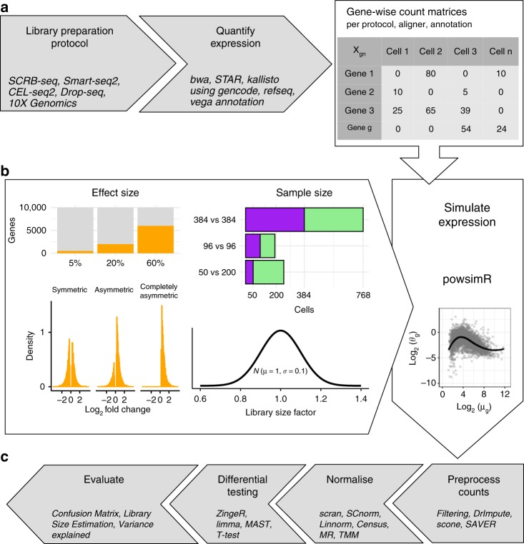
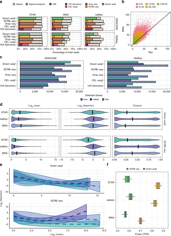
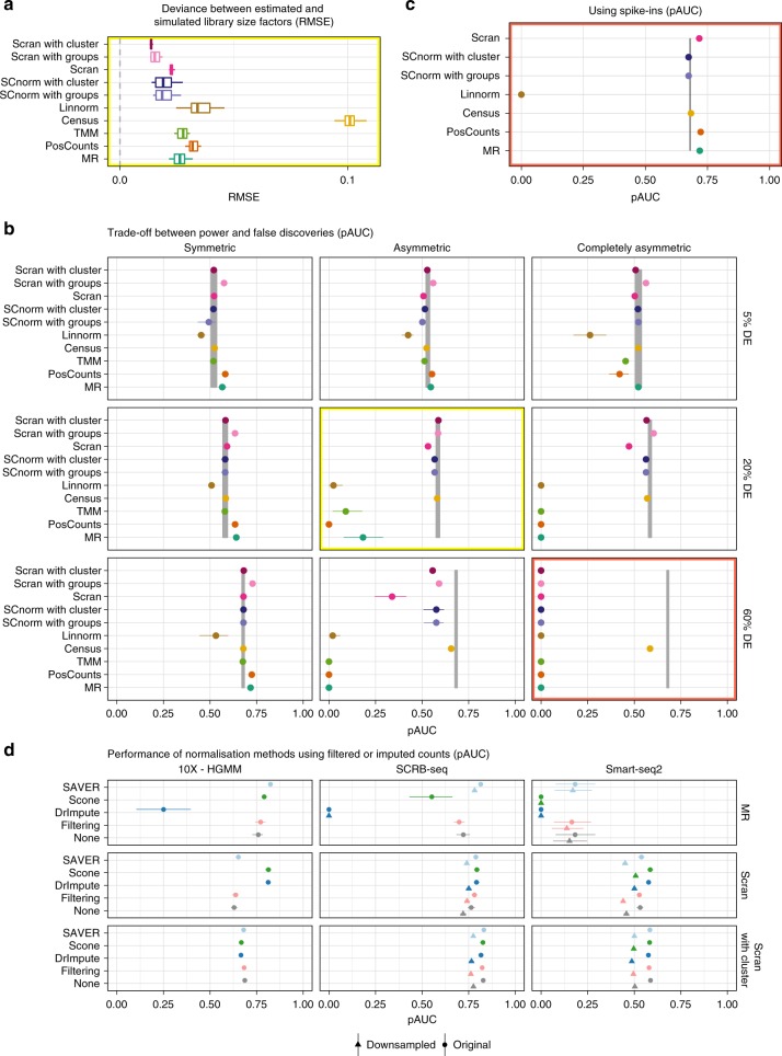
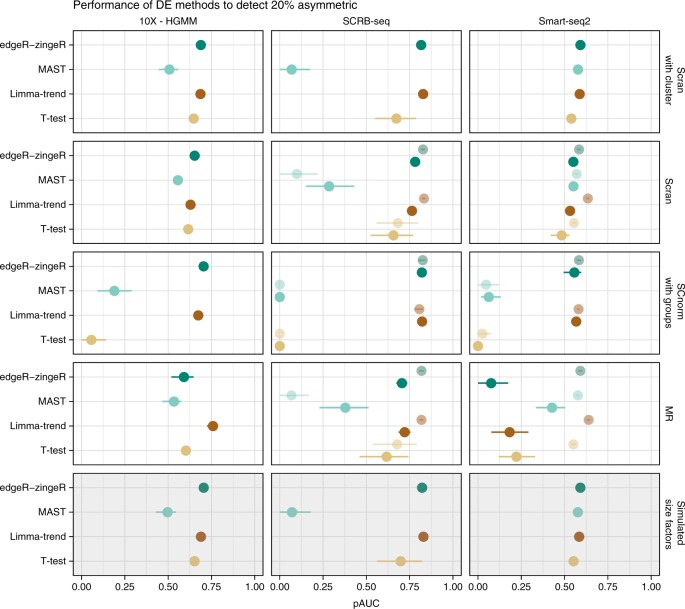
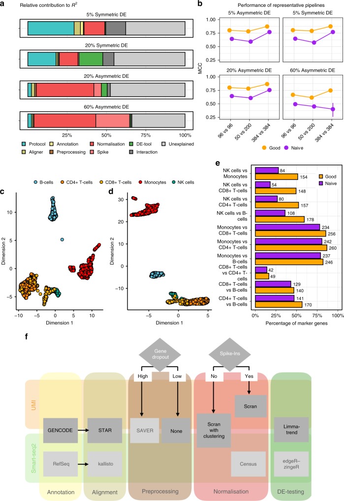
The recent rapid spread of single cell RNA sequencing (scRNA-seq) methods has created a large variety of experimental and computational pipelines for which best practices have not yet been established. Here, we use simulations based on five scRNA-seq library protocols in combination with nine realistic differential expression (DE) setups to systematically evaluate three mapping, four imputation, seven normalisation and four differential expression testing approaches resulting in ~3000 pipelines, allowing us to also assess interactions among pipeline steps. We find that choices of normalisation and library preparation protocols have the biggest impact on scRNA-seq analyses. Specifically, we find that library preparation determines the ability to detect symmetric expression differences, while normalisation dominates pipeline performance in asymmetric DE-setups. Finally, we illustrate the importance of informed choices by showing that a good scRNA-seq pipeline can have the same impact on detecting a biological signal as quadrupling the sample size.
Overview
The claims and statistics of this paper haven’t been checked yet.
Run the check — free, no account needed. It reads the open-access text and checks the sources it cites.
Integrity signals
Registry
Cites
Statistics
Figures
Verification
Claims the paper makes
The claims and statistics of this paper haven’t been checked yet.
Run the check — free, no account needed. It reads the open-access text and checks the sources it cites.
Claims other papers make about this one
Each is checked against this paper’s own text: does it say what the citing paper says it does?
The cited source says what the claim attributes to it.
In the citing paper
“Furthermore, papers evaluating the performance of single-cell-specific tools all compute the simulations as if cells were independent15–21.”
From A practical solution to pseudoreplication bias in single-cell studies (2021) · cites this paper as [15]
In the citing paper
“Scran performs well for batch correction tasks34,35”
From Best practices for single-cell analysis across modalities (2023) · cites this paper as [34]
Self-check
Percentages, sums and reported differences re-computed from the paper’s own numbers.
The self-check needs the paper’s full text.
Citations
Cites
Fast and accurate short read alignment with Burrows-Wheeler transform
Li, H., & Durbin, R. (2009) · Bioinformatics · doi:10.1093/bioinformatics/btp324 · Cited by 58,607
STAR: ultrafast universal RNA-seq aligner
Dobin, A., Davis, C. A., Schlesinger, F., Drenkow, J., Zaleski, C., Jha, S., Batut, P., Chaisson, M., & Gingeras, T. R. (2013) · Bioinformatics · doi:10.1093/bioinformatics/bts635 · Cited by 51,709
Modern Applied Statistics with S
Venables, W. N., & Ripley, B. D. (2002) · Statisctics and computing/Statistics and computing · doi:10.1007/978-0-387-21706-2 · Cited by 25,941
Differential expression analysis for sequence count data
Anders, S., & Huber, W. (2010) · Genome Biology · doi:10.1186/gb-2010-11-10-r106 · Cited by 15,581
Near-optimal probabilistic RNA-seq quantification
Bray, N. L., Pimentel, H., Melsted, P., & Pachter, L. (2016) · Nature Biotechnology · doi:10.1038/nbt.3519 · Cited by 9,723
A scaling normalization method for differential expression analysis of RNA-seq data
Robinson, M. D., & Oshlack, A. (2010) · Genome Biology · doi:10.1186/gb-2010-11-3-r25 · Cited by 7,876
Massively parallel digital transcriptional profiling of single cells
Zheng, G. X. Y., Terry, J. M., Belgrader, P., Ryvkin, P., Bent, Z. W., Wilson, R., Ziraldo, S. B., Wheeler, T. D., McDermott, G. P., Zhu, J., et al. (2017) · Nature Communications · doi:10.1038/ncomms14049 · Cited by 7,353
Highly parallel genome-wide expression profiling of individual cells using nanoliter droplets.
Macosko, E. Z., Basu, A., Satija, R., Nemesh, J., Shekhar, K., Goldman, M., Tirosh, I., Bialas, A. R., Kamitaki, N., Martersteck, E. M., et al. (2015) · Cell · doi:10.1016/j.cell.2015.05.002 · Cited by 7,110
O'Leary, N. A., Wright, M. W., Brister, J. R., Ciufo, S., Haddad, D., McVeigh, R., Rajput, B., Robbertse, B., Smith-White, B., Ako-Adjei, D., et al. (2016) · Nucleic Acids Research · doi:10.1093/nar/gkv1189 · Cited by 6,357
voom: precision weights unlock linear model analysis tools for RNA-seq read counts
Law, C. W., Chen, Y., Shi, W., & Smyth, G. K. (2014) · Genome Biology · doi:10.1186/gb-2014-15-2-r29 · Cited by 6,155
Cited by
Sorted by citations
Eleven grand challenges in single-cell data science
Lähnemann, D., Köster, J., Szczurek, E., McCarthy, D. J., Hicks, S. C., Robinson, M. D., Vallejos, C. A., Campbell, K. R., Beerenwinkel, N., Mahfouz, A., et al. (2020) · Genome Biology · doi:10.1186/s13059-020-1926-6 · Cited by 1,327
Best practices for single-cell analysis across modalities
Heumos, L., Schaar, A. C., Lance, C., Litinetskaya, A., Drost, F., Zappia, L., Lücken, M. D., Strobl, D. C., Henao, J., Curion, F., et al. (2023) · Nature Reviews Genetics · doi:10.1038/s41576-023-00586-w · Cited by 1,051
“…was shown to work better for stabilizing variance for subsequent dimensionality reduction 33 , Scran performs well for batch correction tasks 34,35 , and analytical Pearson residuals are better suited for selection of biologically variable genes and identification of rare cell identities 31…”
BackgroundA Review of Explainable Artificial Intelligence in Healthcare
Sadeghi, Z., Alizadehsani, R., CIFCI, M. A., Kausar, S., Rehman, R., Mahanta, P., Bora, P. K., Almasri, A., Alkhawaldeh, R. S., Hussain, S., et al. (2024) · Computers and Electrical Engineering · doi:10.1016/j.compeleceng.2024.109370 · Cited by 598
Silvin, A., Uderhardt, S., Piot, C., Da Mesquita, S., Yang, K., Geirsdottir, L., Mulder, K., Eyal, D., Liu, Z., Bridlance, C., et al. (2022) · Immunity · doi:10.1016/j.immuni.2022.07.004 · Cited by 368
A practical solution to pseudoreplication bias in single-cell studies
Zimmerman, K. D., Espeland, M. A., & Langefeld, C. D. (2021) · Nature Communications · doi:10.1038/s41467-021-21038-1 · Cited by 356
Single-cell and spatial transcriptomics: deciphering brain complexity in health and disease
Piwecka, M., Rajewsky, N., & Rybak-Wolf, A. (2023) · Nature Reviews Neurology · doi:10.1038/s41582-023-00809-y · Cited by 320
Tutorial: guidelines for the computational analysis of single-cell RNA sequencing data
Andrews, T. S., Kiselev, V. Y., McCarthy, D. J., & Hemberg, M. (2020) · Nature Protocols · doi:10.1038/s41596-020-00409-w · Cited by 323
A systematic evaluation of single-cell RNA-sequencing imputation methods
Hou, W., Ji, Z., Ji, H., & Hicks, S. C. (2020) · Genome biology · doi:10.1186/s13059-020-02132-x · Cited by 307
Single-cell analyses of aging, inflammation and senescence
Uyar, B., Palmer, D. H., Kowald, A., Escobar, H. M., Barrantes, I., Möller, S., Akalin, A., & Fuellen, G. (2020) · Ageing Research Reviews · doi:10.1016/j.arr.2020.101156 · Cited by 207
Applications of single-cell and bulk RNA sequencing in onco-immunology
Kuksin, M., Morel, D., Aglave, M., Danlos, F., Marabelle, A., Zinovyev, A. Y., Gautheret, D., & Verlingue, L. (2021) · European Journal of Cancer · doi:10.1016/j.ejca.2021.03.005 · Cited by 172
Germain, P., Sonrel, A., & Robinson, M. D. (2020) · Genome biology · doi:10.1186/s13059-020-02136-7 · Cited by 157
Cross-species RNA-seq for deciphering host–microbe interactions
Westermann, A. J., & Vogel, J. (2021) · Nature Reviews Genetics · doi:10.1038/s41576-021-00326-y · Cited by 143
Single cell transcriptome profiling of the human alcohol-dependent brain
Brenner, E., Tiwari, G. R., Kapoor, M., Liu, Y., Brock, A., & Mayfield, R. D. (2020) · Human Molecular Genetics · doi:10.1093/hmg/ddaa038 · Cited by 118
DIALOGUE maps multicellular programs in tissue from single-cell or spatial transcriptomics data
Jerby‐Arnon, L., & Regev, A. (2022) · Nature Biotechnology · doi:10.1038/s41587-022-01288-0 · Cited by 119
Gutierrez, C., Al’Khafaji, A. M., Brenner, E. A., Johnson, K. E., Gohil, S. H., Lin, Z., Knisbacher, B. A., Durrett, R., Li, S., Parvin, S., et al. (2021) · Nature Cancer · doi:10.1038/s43018-021-00222-8 · Cited by 109
Junttila, S., Smolander, J., & Elo, L. L. (2022) · Briefings in Bioinformatics · doi:10.1093/bib/bbac286 · Cited by 109
Johnson, K. A., & Krishnan, A. (2022) · Genome biology · doi:10.1186/s13059-021-02568-9 · Cited by 111
Genome-wide kinetic properties of transcriptional bursting in mouse embryonic stem cells
Ochiai, H., Hayashi, T., Umeda, M., Yoshimura, M., Harada, A., Shimizu, Y., Nakano, K., Saitoh, N., Kimura, H., Liu, Z., et al. (2020) · Science Advances · doi:10.1126/sciadv.aaz6699 · Cited by 107
Patch-seq: Past, Present, and Future
Lipovsek, M., Bardy, C., Cadwell, C. R., Hadley, K., Kobak, D., & Tripathy, S. J. (2021) · Journal of Neuroscience · doi:10.1523/jneurosci.1653-20.2020 · Cited by 104
Prime-seq, efficient and powerful bulk RNA sequencing
Janjic, A., Wange, L. E., Bagnoli, J., Geuder, J., Nguyen, P., Richter, D., Vieth, B., Vick, B., Jeremias, I., Ziegenhain, C., et al. (2022) · Genome biology · doi:10.1186/s13059-022-02660-8 · Cited by 99
Self-citationMegakaryocyte and Platelet Transcriptomics for Discoveries in Human Health and Disease
Davizon‐Castillo, P., Rowley, J. W., & Rondina, M. T. (2020) · Arteriosclerosis Thrombosis and Vascular Biology · doi:10.1161/atvbaha.119.313280 · Cited by 96
An AI Agent for Fully Automated Multi‐Omic Analyses
Zhou, J., Zhang, B., Li, G., Chen, X., Li, H., Xu, X., Chen, S., He, W., Xu, C., Liu, L., et al. (2024) · Advanced Science · doi:10.1002/advs.202407094 · Cited by 104
Computational Methods for Single-Cell RNA Sequencing
Hie, B., Peters, J. M., Nyquist, S. K., Shalek, A. K., Berger, B., & Bryson, B. D. (2020) · Annual Review of Biomedical Data Science · doi:10.1146/annurev-biodatasci-012220-100601 · Cited by 89
Koopmans, F., Li, K. W., Klaassen, R. V., & Smit, A. B. (2022) · Journal of Proteome Research · doi:10.1021/acs.jproteome.2c00513 · Cited by 101
Sampling time-dependent artifacts in single-cell genomics studies
Massoni-Badosa, R., Iacono, G., Moutinho, C., Kulis, M., Palau, N., Marchese, D., Rodríguez‐Ubreva, J., Ballestar, E., Rodríguez-Esteban, G., Marsal, S., et al. (2020) · Genome biology · doi:10.1186/s13059-020-02032-0 · Cited by 84
Nkongolo, S., Mahamed, D., Kuipery, A., Vásquez, J. D. S., Kim, S., Mehrotra, A., Patel, A. B., Hu, C., McGilvray, I. D., Feld, J. J., et al. (2023) · Journal of Clinical Investigation · doi:10.1172/jci158903 · Cited by 83
Single cell transcriptome research in human placenta
Li, H., Huang, Q., Liu, Y., & Garmire, L. X. (2020) · Reproduction · doi:10.1530/rep-20-0231 · Cited by 77
A benchmark study of simulation methods for single-cell RNA sequencing data
Cao, Y., Yang, P., & Yang, J. Y. H. (2021) · Nature Communications · doi:10.1038/s41467-021-27130-w · Cited by 76
Optimizing expression quantitative trait locus mapping workflows for single-cell studies
Cuomo, A. S. E., Alvari, G., Azodi, C. B. D., McCarthy, D. J., & Bonder, M. J. (2021) · Genome biology · doi:10.1186/s13059-021-02407-x · Cited by 73
Ko, K. I., Merlet, J., DerGarabedian, B. P., Huang, Z., Suzuki-Horiuchi, Y., Hedberg, M. L., Hu, E. Y., Nguyen, A., Prouty, S. M., Alawi, F., et al. (2022) · Science Translational Medicine · doi:10.1126/scitranslmed.abj0324 · Cited by 82
Benchmarking UMI-based single-cell RNA-seq preprocessing workflows
You, Y., Tian, L., Su, S., Dong, X., Jabbari, J. S., Hickey, P. F., & Ritchie, M. E. (2021) · Genome biology · doi:10.1186/s13059-021-02552-3 · Cited by 77
Critical downstream analysis steps for single-cell RNA sequencing data
Zhang, Z., Cui, F., Lin, C., Zhao, L., Wang, C., & Zou, Q. (2021) · Briefings in Bioinformatics · doi:10.1093/bib/bbab105 · Cited by 72
Durán, R. C., González-Orozco, J. C., Velasco, I., & Wu, J. Q. (2022) · Frontiers in Cell and Developmental Biology · doi:10.3389/fcell.2022.884748 · Cited by 64
To the proteome and beyond: advances in single-cell omics profiling for plant systems
Clark, N. M., Elmore, J. M., & Walley, J. W. (2021) · PLANT PHYSIOLOGY · doi:10.1093/plphys/kiab429 · Cited by 66
Considerations for building and using integrated single-cell atlases
Hrovatin, K., Sikkema, L., Shitov, V. A., Heimberg, G., Shulman, M., Oliver, A. J., Mueller, M. F., Ibarra, I. L., Wang, H., Ramírez-Suástegui, C., et al. (2024) · Nature Methods · doi:10.1038/s41592-024-02532-y · Cited by 72
Baruzzo, G., Cesaro, G., & Camillo, B. D. (2022) · Bioinformatics · doi:10.1093/bioinformatics/btac036 · Cited by 63
Quantitative single-cell transcriptomics
Ziegenhain, C., Vieth, B., Parekh, S., Hellmann, I., & Enard, W. (2018) · Briefings in Functional Genomics · doi:10.1093/bfgp/ely009 · Cited by 60
Self-citationSingle‐Cell Sequencing Methodologies: From Transcriptome to Multi‐Dimensional Measurement
Chen, Y., Song, J. T., Ruan, Q., Zeng, X., Wu, L., Cai, L., Wang, X., & Yang, C. J. (2021) · Small Methods · doi:10.1002/smtd.202100111 · Cited by 61
A hitchhiker's guide to single-cell transcriptomics and data analysis pipelines
Nayak, R., & Hasija, Y. (2021) · Genomics · doi:10.1016/j.ygeno.2021.01.007 · Cited by 62
A review of computational strategies for denoising and imputation of single-cell transcriptomic data
Patruno, L., Maspero, D., Craighero, F., Angaroni, F., Antoniotti, M., & Graudenzi, A. (2020) · Briefings in Bioinformatics · doi:10.1093/bib/bbaa222 · Cited by 56
Inflammatory Bowel Disease Through the Lens of Single-cell RNA-seq Technologies
Corridoni, D., Chapman, T., Antanaviciute, A., Satsangi, J. J., & Simmons, A. (2020) · Inflammatory Bowel Diseases · doi:10.1093/ibd/izaa089 · Cited by 55
Statistical and Bioinformatics Analysis of Data from Bulk and Single-Cell RNA Sequencing Experiments
Yu, X., Aghababazadeh, F. A., Chen, Y. A., & Fridley, B. L. (2020) · Methods in molecular biology · doi:10.1007/978-1-0716-0849-4_9 · Cited by 55
Maden, S. K., Kwon, S. H., Huuki-Myers, L. A., Collado‐Torres, L., Hicks, S. C., & Maynard, K. R. (2023) · Genome biology · doi:10.1186/s13059-023-03123-4 · Cited by 58
Evaluation of STAR and Kallisto on Single Cell RNA-Seq Data Alignment
Du, Y., Huang, Q., Arisdakessian, C. G., & Garmire, L. X. (2020) · G3 Genes Genomes Genetics · doi:10.1534/g3.120.401160 · Cited by 56
Does Gene Expression Noise Play a Functional Role in Plants?
Cortijo, S., & Locke, J. C. W. (2020) · Trends in Plant Science · doi:10.1016/j.tplants.2020.04.017 · Cited by 50
Consensus clustering of single-cell RNA-seq data by enhancing network affinity
Cui, Y., Zhang, S., Liang, Y. J., Wang, X., Ferraro, T. N., & Chen, Y. (2021) · Briefings in Bioinformatics · doi:10.1093/bib/bbab236 · Cited by 51
Riccetti, M., Gokey, J. J., Aronow, B. J., & Perl, A. T. (2020) · Matrix Biology · doi:10.1016/j.matbio.2020.05.002 · Cited by 50
Chen, L., Zhai, Y., He, Q., Wang, W., & Deng, M. (2020) · Genes · doi:10.3390/genes11070792 · Cited by 48
Angiogenesis in Lymph Nodes Is a Critical Regulator of Immune Response and Lymphoma Growth
Menzel, L., Höpken, U. E., & Rehm, A. (2020) · Frontiers in Immunology · doi:10.3389/fimmu.2020.591741 · Cited by 50
Evaluating imputation methods for single-cell RNA-seq data
Yi, C. X., Ma, X., Yuan, L., Sun, Z., & Wang, P. (2023) · BMC Bioinformatics · doi:10.1186/s12859-023-05417-7 · Cited by 51
The shaky foundations of simulating single-cell RNA sequencing data
Crowell, H. L., Leonardo, S. X. M., Soneson, C., & Robinson, M. D. (2023) · Genome biology · doi:10.1186/s13059-023-02904-1 · Cited by 60
Comparative analysis of common alignment tools for single-cell RNA sequencing
Brüning, R. S., Tombor, L. S., Schulz, M. H., Dimmeler, S., & John, D. (2022) · GigaScience · doi:10.1093/gigascience/giac001 · Cited by 43
Machine learning for single-cell genomics data analysis
Raimundo, F., Meng-Papaxanthos, L., Vallot, C., & Vert, J. (2021) · Current Opinion in Systems Biology · doi:10.1016/j.coisb.2021.04.006 · Cited by 46
Toward a Consensus in the Repertoire of Hemocytes Identified in Drosophila
Cattenoz, P. B., Monticelli, S., Pavlidaki, A., & Giangrande, A. (2021) · Frontiers in Cell and Developmental Biology · doi:10.3389/fcell.2021.643712 · Cited by 39
Intraocular dendritic cells characterize HLA-B27-associated acute anterior uveitis
Kasper, M., Heming, M., Schafflick, D., Li, X., Lautwein, T., zu Horste, M. M., Bauer, D., Walscheid, K., Wiendl, H., Loser, K., et al. (2021) · eLife · doi:10.7554/elife.67396 · Cited by 38
Deep learning-based advances and applications for single-cell RNA-sequencing data analysis
Bao, S., Li, K., Yan, C., Zhang, Z., Qu, J., & Zhou, M. (2021) · Briefings in Bioinformatics · doi:10.1093/bib/bbab473 · Cited by 40
Soraggi, S., Riera, M., Meyts, E. R., Schierup, M. H., & Almstrup, K. (2020) · Human Genetics · doi:10.1007/s00439-020-02116-8 · Cited by 36
Göcz, B., Rumpler, É., Sárvári, M., Skrapits, K., Takács, S., Farkas, I., Csillag, V., Trinh, S. H., Bardóczi, Z., Ruska, Y., et al. (2022) · Proceedings of the National Academy of Sciences · doi:10.1073/pnas.2113749119 · Cited by 35
Xiong, Z., Yang, Q., & Li, X. (2020) · CNS Neuroscience & Therapeutics · doi:10.1111/cns.13396 · Cited by 36
Johnson, K. E., Howard, G. R., Morgan, D., Brenner, E. A., Gardner, A. L., Durrett, R., Mo, W., Al’Khafaji, A. M., Sontag, E. D., Jarrett, A. M., et al. (2020) · Physical Biology · doi:10.1088/1478-3975/abb09c · Cited by 35
NECAB1 and NECAB2 are Prevalent Calcium-Binding Proteins of CB1/CCK-Positive GABAergic Interneurons
Miczán, V., Kelemen, K., Glavinics, J. R., László, Z. I., Barti, B., Kenesei, K., Kisfali, M., & Katona, I. (2020) · Cerebral Cortex · doi:10.1093/cercor/bhaa326 · Cited by 30
Sokolowski, D., Faykoo-Martinez, M., Erdman, L., Hou, H., Chan, C., Zhu, H., Holmes, M. M., Goldenberg, A., & Wilson, M. D. (2021) · NAR Genomics and Bioinformatics · doi:10.1093/nargab/lqab011 · Cited by 32
Canozo, F. J. G., Zuo, Z. C., Martin, J. F., & Samee, M. A. H. (2021) · Cell Systems · doi:10.1016/j.cels.2021.09.004 · Cited by 34
Perspectives on rigor and reproducibility in single cell genomics
Gibson, G. C. (2022) · PLoS Genetics · doi:10.1371/journal.pgen.1010210 · Cited by 31
Single-Cell Sequencing: Genomic and Transcriptomic Approaches in Cancer Cell Biology
Ortega-Batista, A., Jaén-Alvarado, Y., Moreno-Labrador, D., Gómez, N., García, G., & Guerrero, E. N. (2025) · International Journal of Molecular Sciences · doi:10.3390/ijms26052074 · Cited by 37
Durán, R. C., Wei, H., & Wu, J. (2024) · BMC Genomics · doi:10.1186/s12864-024-10364-5 · Cited by 37
Cho, J., Kim, S., Lee, H., Rah, W., Cho, H. C., Kim, N. K., Bae, S., Shin, D. H., Lee, M. G., Park, I., et al. (2021) · Nature Biomedical Engineering · doi:10.1038/s41551-021-00783-0 · Cited by 33
From multitude to singularity: An up-to-date overview of scRNA-seq data generation and analysis
Carangelo, G., Magi, A., & Semeraro, R. (2022) · Frontiers in Genetics · doi:10.3389/fgene.2022.994069 · Cited by 39
Osthege, M., Tenhaef, N., Zyla, R., Müller, C., Hemmerich, J., Wiechert, W., Noack, S., & Oldiges, M. (2022) · Engineering in Life Sciences · doi:10.1002/elsc.202100108 · Cited by 32
Tuning parameters of dimensionality reduction methods for single-cell RNA-seq analysis
Raimundo, F., Vallot, C., & Vert, J. (2020) · Genome biology · doi:10.1186/s13059-020-02128-7 · Cited by 33
Li, M., Nishimura, T., Takeuchi, Y., Hongu, T., Wang, Y., Shiokawa, D., Wang, K., Hirose, H., Sasahara, A., Yano, M., et al. (2023) · Journal of Clinical Investigation · doi:10.1172/jci166666 · Cited by 30
Tfh Cells in Health and Immunity: Potential Targets for Systems Biology Approaches to Vaccination
Law, H. L., Venturi, V., Kelleher, A. D., & Munier, C. M. L. (2020) · International Journal of Molecular Sciences · doi:10.3390/ijms21228524 · Cited by 30
CSEA-DB: an omnibus for human complex trait and cell type associations
Dai, Y., Hu, R., Manuel, A. M., Liu, A., Jia, P., & Zhao, Z. (2020) · Nucleic Acids Research · doi:10.1093/nar/gkaa1064 · Cited by 31
Integration of Computational Analysis and Spatial Transcriptomics in Single-Cell Studies
Wang, R., Peng, G., Tam, P., & Jing, N. (2022) · Genomics Proteomics & Bioinformatics · doi:10.1016/j.gpb.2022.06.006 · Cited by 26
The circadian clock is disrupted in pancreatic cancer
Schwartz, P. B., Nukaya, M., Berres, M. E., Rubinstein, C. D., Wu, G., Hogenesch, J. B., Bradfield, C. A., & Ronnekleiv‐Kelly, S. M. (2023) · PLoS Genetics · doi:10.1371/journal.pgen.1010770 · Cited by 28
Thurman, A. L., Ratcliff, J. A., Chimenti, M. S., & Pezzulo, A. A. (2021) · Bioinformatics · doi:10.1093/bioinformatics/btab337 · Cited by 27
RNA recording in single bacterial cells using reprogrammed tracrRNAs
Jiao, C., Reckstadt, C., König, F., Homberger, C., Yu, J., Vogel, J., Westermann, A. J., Sharma, C. M., & Beisel, C. L. (2023) · Nature Biotechnology · doi:10.1038/s41587-022-01604-8 · Cited by 28
Meng, F.-L., Huang, X., Qin, W., Liu, K.-B., Wang, Y., Li, M., Ren, Y., Li, Y.-Z., & Sun, Y. (2023) · Biomarker Research · doi:10.1186/s40364-023-00523-3 · Cited by 27
Comparison of high-throughput single-cell RNA sequencing data processing pipelines
Gao, M., Ling, M., Tang, X., Wang, S., Xu, X., Qiao, Y., Yang, W., & Yu, R. (2020) · Briefings in Bioinformatics · doi:10.1093/bib/bbaa116 · Cited by 24
Taming human brain organoids one cell at a time
Atamian, A., Cordón-Barris, L., & Quadrato, G. (2020) · Seminars in Cell and Developmental Biology · doi:10.1016/j.semcdb.2020.05.022 · Cited by 26
Zhang, X., Lai, H., Zhang, F., Wang, Y., Zhang, L., Yang, N., Wang, C., Liang, Z., Zeng, J., & Yang, J. (2021) · Frontiers in Medicine · doi:10.3389/fmed.2021.635035 · Cited by 25
The accuracy of absolute differential abundance analysis from relative count data
Roche, K. E., & Mukherjee, S. (2022) · PLoS Computational Biology · doi:10.1371/journal.pcbi.1010284 · Cited by 22
Brandt, L., Cristinelli, S., & Ciuffi, A. (2020) · Annual Review of Virology · doi:10.1146/annurev-virology-021820-102458 · Cited by 25
Wang, L., Xie, Y., Chen, W., Zhang, Y., & Zeng, Y. (2021) · Animal Bioscience · doi:10.5713/ab.21.0092 · Cited by 24
COTAN: scRNA-seq data analysis based on gene co-expression
Galfrè, S. G., Morandin, F., Pietrosanto, M., Cremisi, F., & Helmer‐Citterich, M. (2021) · NAR Genomics and Bioinformatics · doi:10.1093/nargab/lqab072 · Cited by 24
AdRoit is an accurate and robust method to infer complex transcriptome composition
Yang, T., Alessandri‐Haber, N., Fury, W., Schaner, M., Breese, R., LaCroix‐Fralish, M. L., Kim, J., Adler, C., Macdonald, L. E., Atwal, G. S., et al. (2021) · Communications Biology · doi:10.1038/s42003-021-02739-1 · Cited by 23
Mahdipour–Shirayeh, A., Erdmann, N., Leung-Hagesteijn, C., & Tiedemann, R. E. (2021) · Briefings in Bioinformatics · doi:10.1093/bib/bbab413 · Cited by 25
Effect of imputation on gene network reconstruction from single-cell RNA-seq data
Ly, L.-H., & Vingron, M. (2021) · Patterns · doi:10.1016/j.patter.2021.100414 · Cited by 24
Differential expression analysis using a model-based gene clustering algorithm for RNA-seq data
Osabe, T., Shimizu, K., & Kadota, K. (2021) · BMC Bioinformatics · doi:10.1186/s12859-021-04438-4 · Cited by 25
Nault, R., Saha, S., Bhattacharya, S., Dodson, J. P., Sinha, S., Maiti, T., & Zacharewski, T. R. (2022) · Nucleic Acids Research · doi:10.1093/nar/gkac019 · Cited by 20
Borsi, G., Motheramgari, K., Dhiman, H., Baumann, M., Sinkala, E., Sauerland, M. B., Riba, J., & Borth, N. (2023) · Journal of Biotechnology · doi:10.1016/j.jbiotec.2023.01.006 · Cited by 20
Houser, A. E., Kazmi, A., Nair, A., & Ji, A. L. (2023) · JID Innovations · doi:10.1016/j.xjidi.2023.100198 · Cited by 23
An era of single-cell genomics consortia
Ando, Y., Kwon, A. T.-J., & Shin, J. W. (2020) · Experimental & Molecular Medicine · doi:10.1038/s12276-020-0409-x · Cited by 20
Yuan, F., Li, Y., Hu, R., Gong, M., Chai, M., Ma, X., Cha, J., Guo, P., Yang, K., Li, M., et al. (2023) · Molecular Psychiatry · doi:10.1038/s41380-023-01987-3 · Cited by 20
High-throughput full-length single-cell RNA-seq automation
Mamanova, L., Miao, Z., Jinat, A., Ellis, P., Shirley, L., & Teichmann, S. A. (2021) · Nature Protocols · doi:10.1038/s41596-021-00523-3 · Cited by 18
scGAD: a new task and end-to-end framework for generalized cell type annotation and discovery
Zhai, Y., Chen, L., & Deng, M. (2023) · Briefings in Bioinformatics · doi:10.1093/bib/bbad045 · Cited by 17
Uncovering functional lncRNAs by scRNA-seq with ELATUS
Goñi, E., Mas, A. M., González, J., Abad, A., Santisteban, M., Fortes, P., Huarte, M., & Hernáez, M. (2024) · Nature Communications · doi:10.1038/s41467-024-54005-7 · Cited by 17
Krzak, M., Alegbe, T., Taylor, D., Ghouraba, M., Strickland, M., Satti, R., Thompson, T., Arestang, K., Przybilla, M., Ramirez-Navarro, L., et al. (2023) · medRxiv · doi:10.1101/2023.09.06.23295056 · Cited by 3
Key Considerations on CITE‐Seq for Single‐Cell Multiomics
Song, H.-W., Martin, J., Shi, X., & Tyznik, A. J. (2025) · PROTEOMICS · doi:10.1002/pmic.202400011 · Cited by 20
Multi-Omics Profiling of the Tumor Microenvironment
Oekelen, O. V., & Laganà, A. (2022) · Advances in experimental medicine and biology · doi:10.1007/978-3-030-91836-1_16 · Cited by 13
Metadata
- Authors
- Vieth, B., Parekh, S., Ziegenhain, C., Enard, W., & Hellmann, I.
- Affiliations
- Ludwig-Maximilians-Universität München (DE)
- Max Planck Institute for Biology of Ageing (DE)
- Karolinska Institutet (SE)
- Corresponding author
- Hellmann, Ines
- Venue
- Nature Communications
- Published
- 2019-10-11
- Volume
- 10
- Issue
- 1
- Pages
- 4667-4667
- ISSN
- 2041-1723 (ISSN-L)
- PMC
- PMC6789098
- OpenAlex
- W2980147288
- Cited by
- 265
- References
- 59
- Citations by year
- 2026: 10 · 2025: 13 · 2024: 24 · 2023: 41 · 2022: 38 · 2021: 82 · 2020: 55 · 2019: 1
- FWCI
- 15.38
- Type
- journal article
- Language
- en
- Open access
- gold
- doi.org
- Locations
- Nature Communications (publishedVersion, cc-by)
- bioRxiv (Cold Spring Harbor Laboratory) (acceptedVersion, cc-by-nc-nd)
- PubMed Central (publishedVersion, cc-by)
- PubMed (publishedVersion)
- RePEc: Research Papers in Economics (submittedVersion)
- DOAJ (DOAJ: Directory of Open Access Journals) (submittedVersion, cc-by-sa)
- DOAJ (DOAJ: Directory of Open Access Journals) (submittedVersion)
- Open access LMU (Ludwid Maxmilian's Universitat Munchen) (submittedVersion, cc-by)
- Funders
- Deutsche Forschungsgemeinschaft (SFB 1243)
- Topics
- Life Sciences › Biochemistry, Genetics and Molecular Biology › Molecular Biology › Single-cell and spatial transcriptomics
- Life Sciences › Biochemistry, Genetics and Molecular Biology › Molecular Biology › Gene expression and cancer classification
- Life Sciences › Biochemistry, Genetics and Molecular Biology › Molecular Biology › Genomics and Phylogenetic Studies
- Keywords
- single-cell RNA sequencing, data analysis pipeline, differential gene expression, library preparation protocols, normalization, imputation, read mapping, simulated data, sample size, best practices
- MeSH terms
- RNA-Seq, Animals, Electronic Data Processing, Chromosome Mapping, Computer Simulation, Mice, Single-Cell Analysis
About these checks
Registry, retraction, Cites and statistics results are computed, not judged, with one exception: a printed reference that no index lists is read once by a model before it counts as a citation error. Claims are extracted by a model and kept only when their quote appears verbatim in the text; each cited source is then checked, with a model’s help, for whether it says what the claim relies on. Those verdicts can be wrong — read the claim’s quote and the cited source before relying on one.
Statistics and arithmetic are recomputed, not judged.
Confidence bands are shown only for fields calibrated on our annotated test set. None is calibrated yet, so no band is shown.
What counts as a claim ›How we measure confidence ›How we check this ›
Are you an author, or do you see a problem with this page? Request a review
