Cited by 31Visual perception and processing mechanismsDecision-Making and Behavioral EconomicsNeural and Behavioral Psychology Studies

The DOI matches its Crossref record; 71 of the 71 references it cites were found in a registry or an index.

Natural statistics support a rational account of confidence biases

Open access

Published version of a preprint

Abstract

Previous work has sought to understand decision confidence as a prediction of the probability that a decision will be correct, leading to debate over whether these predictions are optimal, and whether they rely on the same decision variable as decisions themselves. This work has generally relied on idealized, low-dimensional models, necessitating strong assumptions about the representations over which confidence is computed. To address this, we used deep neural networks to develop a model of decision confidence that operates directly over high-dimensional, naturalistic stimuli. The model accounts for a number of puzzling dissociations between decisions and confidence, reveals a rational explanation of these dissociations in terms of optimization for the statistics of sensory inputs, and makes the surprising prediction that, despite these dissociations, decisions and confidence depend on a common decision variable.

Overview

The claims and statistics of this paper haven’t been checked yet.

Run the check — free, no account needed. It reads the open-access text and checks the sources it cites.

A few free checks a day · papers already verified open instantly · results are public

Integrity signals

Registry

Crossref · 10.1038/s41467-023-39737-2

Cites

71 of 71 references verified0 citation errors · 0 not checkable

Statistics

Figures

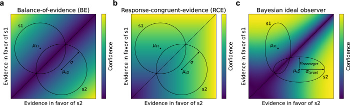
Fig. 1 Detection-theoretic formalization of confidence in two-choice tasks. a Stimuli are modeled as samples from two-dimensional Gaussian distributions (with means μs1 and μs2, and variance σ), schematized as circles labeled s1 and s2, where each dimension represents the evidence in favor of one stimulus category. Given these assumptions, the optimal procedure for estimating confidence is a balance-of-evidence (BE) rule, based on the difference between the evidence in favor of s1 and s2. b Many results are well modeled by an alternative response-congruent-evidence (RCE) heuristic, according to which, after making a decision, confidence is based entirely on the evidence in favor of the chosen stimulus category, ignoring the evidence in favor of the alternative choice. c Bayesian ideal observer with alternative variance assumptions. When stimulus distributions are characterized by greater variance in the dimension in favor of the correct answer (σtarget) than the dimension in favor of the incorrect answer (σnontarget), as proposed in refs. 18 and 19, the optimal procedure for estimating confidence involves a more complex function.
Fig. 1 Detection-theoretic formalization of confidence in two-choice tasks. a Stimuli are modeled as samples from two-dimensional Gaussian distributions (with means μs1 and μs2, and variance σ), schematized as circles labeled s1 and s2, where each dimension represents the evidence in favor of one stimulus category. Given these assumptions, the optimal procedure for estimating confidence is a balance-of-evidence (BE) rule, based on the difference between the evidence in favor of s1 and s2. b Many results are well modeled by an alternative response-congruent-evidence (RCE) heuristic, according to which, after making a decision, confidence is based entirely on the evidence in favor of the chosen stimulus category, ignoring the evidence in favor of the alternative choice. c Bayesian ideal observer with alternative variance assumptions. When stimulus distributions are characterized by greater variance in the dimension in favor of the correct answer (σtarget) than the dimension in favor of the incorrect answer (σnontarget), as proposed in refs. 18 and 19, the optimal procedure for estimating confidence involves a more complex function.CC BY · PubMed Central
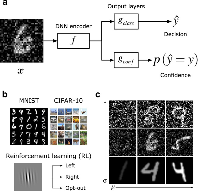
Fig. 2 Performance-optimized neural network model of decision confidence. a Model architecture. An image x, belonging to class y, was passed through a deep neural network (DNN) encoder f (the exact architecture of this encoder depended on the dataset, as detailed in “Encoder”), followed by two output layers: gclass generated a decision y^ classifying the image, and gconf generated a confidence score by predicting p(y^=y), the probability that the decision was correct. b The model was trained through supervised learning using the MNIST handwritten digits dataset and the CIFAR-10 object classification dataset. For these datasets, the classification layer was trained to label the class of the image, and the confidence layer was trained to output a target of 1 if the classification response was correct, and 0 if the classification response was incorrect. The model was also trained through reinforcement learning (RL) to perform an orientation discrimination task, in which, rather than generating an explicit confidence rating, the model had the option to opt-out of a decision and receive a small but guaranteed reward, allowing the use of the opt-out rate as an implicit measure of confidence. c To evaluate the relative influence of signal strength and noise on the model’s behavior, images were modified by manipulating both the contrast μ and the noise level σ.
Fig. 2 Performance-optimized neural network model of decision confidence. a Model architecture. An image x, belonging to class y, was passed through a deep neural network (DNN) encoder f (the exact architecture of this encoder depended on the dataset, as detailed in “Encoder”), followed by two output layers: gclass generated a decision y^ classifying the image, and gconf generated a confidence score by predicting p(y^=y), the probability that the decision was correct. b The model was trained through supervised learning using the MNIST handwritten digits dataset and the CIFAR-10 object classification dataset. For these datasets, the classification layer was trained to label the class of the image, and the confidence layer was trained to output a target of 1 if the classification response was correct, and 0 if the classification response was incorrect. The model was also trained through reinforcement learning (RL) to perform an orientation discrimination task, in which, rather than generating an explicit confidence rating, the model had the option to opt-out of a decision and receive a small but guaranteed reward, allowing the use of the opt-out rate as an implicit measure of confidence. c To evaluate the relative influence of signal strength and noise on the model’s behavior, images were modified by manipulating both the contrast μ and the noise level σ.CC BY · PubMed Central
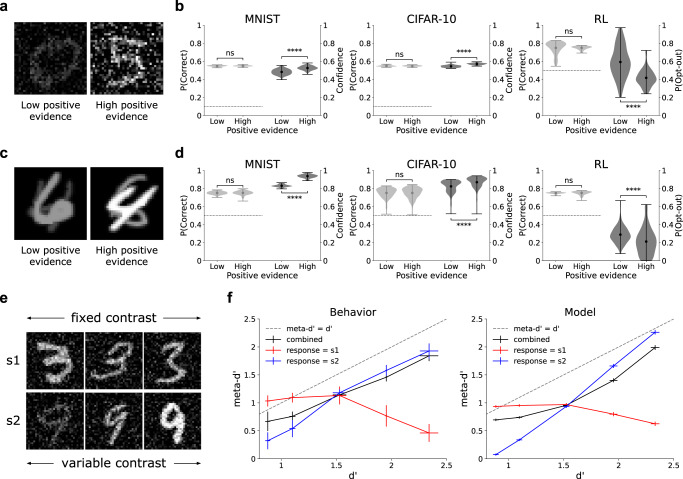
Fig. 3 Behavioral dissociations between decisions and confidence. a Human and animal decision confidence displays a positive evidence (PE) bias: higher confidence (or lower opt-out rate) in the high vs. low PE conditions despite balanced signal-to-noise ratio and balanced decision accuracy. b The PE bias naturally emerges in performance-optimized neural networks across multiple datasets, architectures, and learning paradigms (two-sided paired t-tests; accuracy: MNIST, p = 0.42; CIFAR-10, p = 0.48; RL, p = 0.97; confidence: MNIST, p = 1.4 × 10⁻²⁰; CIFAR-10, p = 4.3 × 10−50; RL, p = 4.4 × 10⁻²⁰). See Supplementary Fig. S1 for confidence distributions in correct vs. incorrect trials. Note that stimulus parameters (contrast and noise) were set so as to target the threshold between chance performance (dotted black lines) and 100% accuracy, resulting in ~ 55% accuracy for 10-choice tasks and ~ 75% accuracy for two-choice tasks. The model achieved much higher accuracy when presented with noiseless images (96.3% ± 0.03 for MNIST, 88.1% ± 0.05 for CIFAR-10). c An alternative test for the PE bias, involving superimposed stimuli presented at different contrast levels, where the task is to indicate which stimulus is presented at a higher contrast. In the high positive evidence condition, there is both higher positive evidence (evidence in favor of the correct answer, 4 in this case), and higher negative evidence (evidence in favor of the incorrect answer, 6 in this case), than in the low positive evidence condition. Visual noise was also included in images, but is omitted here for clarity of visualization. d The model also shows this alternative formulation of the PE bias (two-sided paired t-tests; accuracy: MNIST, p = 0.8; CIFAR-10, p = 0.99; RL, p = 0.83; confidence: MNIST, p = 8.3 × 10−84; CIFAR-10, p = 2.8 × 10−48; RL, p = 2.8 × 10⁻¹⁰). e Adaptation of behavioral paradigm from Maniscalco et al.13, s1 is presented at an intermediate contrast, while the contrast of s2 is varied. f This produces a strong dissociation between type-1 sensitivity (d') and type-2 sensitivity (meta-d'): when participants respond s1, meta-d' decreases as d' increases (Behavior), a phenomenon which is captured by the neural network model (Model). Results in (b) and (d) reflect probability density over 100 trained networks, with mean accuracy/confidence in each condition represented by circular markers, and maxima/minima represented by the upper/lower line; results in (f) reflect mean d'/meta-d' over 100 trained networks ± the standard of the mean; ns indicates p > 0.05, ****p < 0.0001. Source data are provided as a Source Data file.
Fig. 3 Behavioral dissociations between decisions and confidence. a Human and animal decision confidence displays a positive evidence (PE) bias: higher confidence (or lower opt-out rate) in the high vs. low PE conditions despite balanced signal-to-noise ratio and balanced decision accuracy. b The PE bias naturally emerges in performance-optimized neural networks across multiple datasets, architectures, and learning paradigms (two-sided paired t-tests; accuracy: MNIST, p = 0.42; CIFAR-10, p = 0.48; RL, p = 0.97; confidence: MNIST, p = 1.4 × 10⁻²⁰; CIFAR-10, p = 4.3 × 10−50; RL, p = 4.4 × 10⁻²⁰). See Supplementary Fig. S1 for confidence distributions in correct vs. incorrect trials. Note that stimulus parameters (contrast and noise) were set so as to target the threshold between chance performance (dotted black lines) and 100% accuracy, resulting in ~ 55% accuracy for 10-choice tasks and ~ 75% accuracy for two-choice tasks. The model achieved much higher accuracy when presented with noiseless images (96.3% ± 0.03 for MNIST, 88.1% ± 0.05 for CIFAR-10). c An alternative test for the PE bias, involving superimposed stimuli presented at different contrast levels, where the task is to indicate which stimulus is presented at a higher contrast. In the high positive evidence condition, there is both higher positive evidence (evidence in favor of the correct answer, 4 in this case), and higher negative evidence (evidence in favor of the incorrect answer, 6 in this case), than in the low positive evidence condition. Visual noise was also included in images, but is omitted here for clarity of visualization. d The model also shows this alternative formulation of the PE bias (two-sided paired t-tests; accuracy: MNIST, p = 0.8; CIFAR-10, p = 0.99; RL, p = 0.83; confidence: MNIST, p = 8.3 × 10−84; CIFAR-10, p = 2.8 × 10−48; RL, p = 2.8 × 10⁻¹⁰). e Adaptation of behavioral paradigm from Maniscalco et al.13, s1 is presented at an intermediate contrast, while the contrast of s2 is varied. f This produces a strong dissociation between type-1 sensitivity (d') and type-2 sensitivity (meta-d'): when participants respond s1, meta-d' decreases as d' increases (Behavior), a phenomenon which is captured by the neural network model (Model). Results in (b) and (d) reflect probability density over 100 trained networks, with mean accuracy/confidence in each condition represented by circular markers, and maxima/minima represented by the upper/lower line; results in (f) reflect mean d'/meta-d' over 100 trained networks ± the standard of the mean; ns indicates p > 0.05, ****p < 0.0001. Source data are provided as a Source Data file.CC BY · PubMed Central
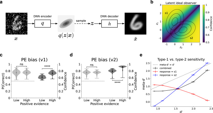
Fig. 4 Latent ideal observer accounts for dissociations between decisions and confidence. a Denoising variational autoencoder (VAE) used to extract low-dimensional latent representation of training data. An image x was passed through a DNN encoder q (distinct from the encoder f used in the supervised neural network model), which output the parameters (means and variances) of the latent posterior q(z∣x), a two-dimensional Gaussian distribution. This distribution was sampled from, yielding z, which was then passed through a DNN decoder h, yielding x~, a denoised reconstruction of the input x. The VAE was regularized based on the divergence of the latent posterior from a unit normal prior (with means equal to 0 and variances equal to 1), encouraging efficient low-dimensional encodings of the high-dimensional inputs. b Latent ideal observer model. After training the VAE, Gaussian distributions were fit to the latent representations resulting from the training images for classes s1 and s2. The distributions were used to construct an ideal observer model that computed confidence according to p(correct∣z), the probability of being correct given the low-dimensional embedding z. Concentric ellipses represent distributions based on the average parameters of those extracted from 100 trained VAEs. The latent ideal observer accounted for both versions of the PE bias, including (c) the version involving manipulation of contrast and noise (Fig. 3a; two-sided paired t-tests, accuracy: p = 0.97, confidence: p = 1.3 × 10−60), and (d) the version involving superimposed stimuli presented at different contrast levels (Fig. 3c; two-sided paired t-tests, accuracy: p = 0.82, confidence: p = 1.3 × 10−62). Confidence for correct and incorrect trials is shown in Supplementary Fig. S3. e The latent ideal observer also accounted for the dissociation between type-1 and type-2 sensitivity. Results in (c) and (d) reflect probability density over 100 ideal observers (each based on distributions extracted by a separate trained VAE), with mean accuracy/confidence in each condition represented by circular markers, and maxima/minima represented by the upper/lower line; Results in (e) reflect mean d'/meta-d' over 100 ideal observers ± the standard of the mean; dotted black lines represent chance performance; ns indicates p > 0.05, ****p < 0.0001. Source data are provided as a Source Data file.
Fig. 4 Latent ideal observer accounts for dissociations between decisions and confidence. a Denoising variational autoencoder (VAE) used to extract low-dimensional latent representation of training data. An image x was passed through a DNN encoder q (distinct from the encoder f used in the supervised neural network model), which output the parameters (means and variances) of the latent posterior q(z∣x), a two-dimensional Gaussian distribution. This distribution was sampled from, yielding z, which was then passed through a DNN decoder h, yielding x~, a denoised reconstruction of the input x. The VAE was regularized based on the divergence of the latent posterior from a unit normal prior (with means equal to 0 and variances equal to 1), encouraging efficient low-dimensional encodings of the high-dimensional inputs. b Latent ideal observer model. After training the VAE, Gaussian distributions were fit to the latent representations resulting from the training images for classes s1 and s2. The distributions were used to construct an ideal observer model that computed confidence according to p(correct∣z), the probability of being correct given the low-dimensional embedding z. Concentric ellipses represent distributions based on the average parameters of those extracted from 100 trained VAEs. The latent ideal observer accounted for both versions of the PE bias, including (c) the version involving manipulation of contrast and noise (Fig. 3a; two-sided paired t-tests, accuracy: p = 0.97, confidence: p = 1.3 × 10−60), and (d) the version involving superimposed stimuli presented at different contrast levels (Fig. 3c; two-sided paired t-tests, accuracy: p = 0.82, confidence: p = 1.3 × 10−62). Confidence for correct and incorrect trials is shown in Supplementary Fig. S3. e The latent ideal observer also accounted for the dissociation between type-1 and type-2 sensitivity. Results in (c) and (d) reflect probability density over 100 ideal observers (each based on distributions extracted by a separate trained VAE), with mean accuracy/confidence in each condition represented by circular markers, and maxima/minima represented by the upper/lower line; Results in (e) reflect mean d'/meta-d' over 100 ideal observers ± the standard of the mean; dotted black lines represent chance performance; ns indicates p > 0.05, ****p < 0.0001. Source data are provided as a Source Data file.CC BY · PubMed Central
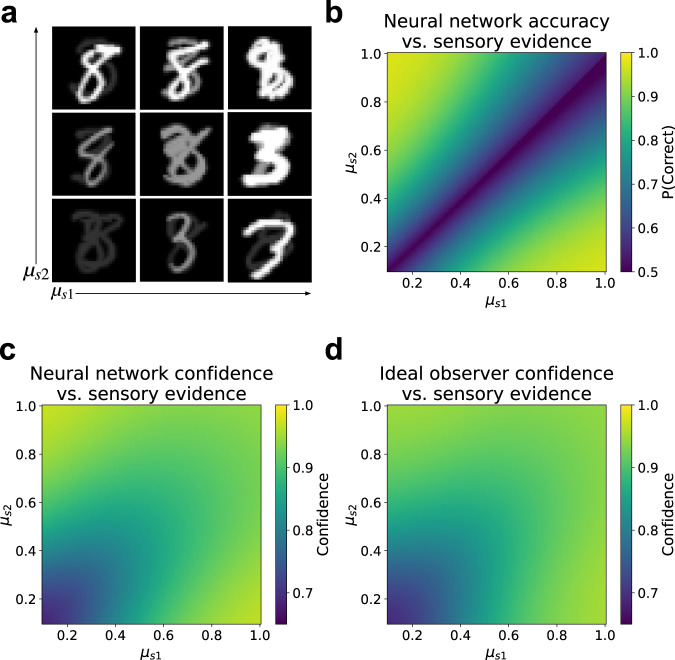
Fig. 5 Learned confidence strategy best explained by ideal observer. a Generalized version of positive evidence manipulation used to comprehensively evaluate both accuracy and confidence as a function of sensory evidence. Model was trained on classification of individual stimuli over the standard range of contrast and noise levels, then tested on images consisting of two superimposed stimuli belonging to classes s1 and s2, with independently varying contrast levels μs1 and μs2 (visual noise was also included in images presented to the model). b Decision accuracy resembled the BE rule, as expected given uniform sampling of sensory evidence space. c Confidence displayed a more complex pattern. d Confidence was best predicted by the latent ideal observer model, which outperformed regression models based on either the RCE or BE rules. Results reflect an average over 100 trained networks. Source data are provided as a Source Data file.
Fig. 5 Learned confidence strategy best explained by ideal observer. a Generalized version of positive evidence manipulation used to comprehensively evaluate both accuracy and confidence as a function of sensory evidence. Model was trained on classification of individual stimuli over the standard range of contrast and noise levels, then tested on images consisting of two superimposed stimuli belonging to classes s1 and s2, with independently varying contrast levels μs1 and μs2 (visual noise was also included in images presented to the model). b Decision accuracy resembled the BE rule, as expected given uniform sampling of sensory evidence space. c Confidence displayed a more complex pattern. d Confidence was best predicted by the latent ideal observer model, which outperformed regression models based on either the RCE or BE rules. Results reflect an average over 100 trained networks. Source data are provided as a Source Data file.CC BY · PubMed Central
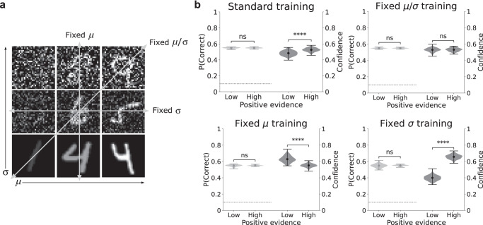
Fig. 6 The PE bias is driven by distribution of training data. a Illustration of four different training regimes. In the standard training regime, the model was trained on the full range of variability in both contrast and noise levels. In the fixed μ/σ regime, the model was trained on images with a fixed signal-to-noise ratio, equivalent to being trained directly on the positive evidence manipulation. In the fixed μ regime, the model was trained on images that varied only in their noise level. In the fixed σ regime, the model was trained on images that varied only in their contrast level. b Effect of training regime on presence of PE bias. Variance in both contrast and noise (standard training) resulted in PE bias (two-sided paired t-tests, accuracy: p = 0.42, confidence: p = 1.4 × 10⁻²⁰). Fixed contrast-to-noise ratio (fixed μ/σ training) resulted in no PE bias (two-sided paired t-tests, accuracy: p = 0.7, confidence: p = 0.31). Variance in noise only (fixed μ training) resulted in reversed PE bias—higher confidence in low vs. high PE conditions (two-sided paired t-tests, accuracy: p = 0.21, confidence: p = 4.8 × 10⁻³⁵). Variance in contrast only (fixed σ training) resulted in significantly larger PE bias than standard training regime (two-sided paired t-tests, accuracy: p = 0.47, confidence: p = 4.8 × 10−79). Results reflect probability density over 100 trained networks, with mean accuracy/confidence in each condition represented by circular markers, and maxima/minima represented by the upper/lower line; ns indicates p > 0.05, ****p < 0.0001. Confidence for correct and incorrect trials is shown in Supplementary Fig. S6. Source data are provided as a Source Data file.
Fig. 6 The PE bias is driven by distribution of training data. a Illustration of four different training regimes. In the standard training regime, the model was trained on the full range of variability in both contrast and noise levels. In the fixed μ/σ regime, the model was trained on images with a fixed signal-to-noise ratio, equivalent to being trained directly on the positive evidence manipulation. In the fixed μ regime, the model was trained on images that varied only in their noise level. In the fixed σ regime, the model was trained on images that varied only in their contrast level. b Effect of training regime on presence of PE bias. Variance in both contrast and noise (standard training) resulted in PE bias (two-sided paired t-tests, accuracy: p = 0.42, confidence: p = 1.4 × 10⁻²⁰). Fixed contrast-to-noise ratio (fixed μ/σ training) resulted in no PE bias (two-sided paired t-tests, accuracy: p = 0.7, confidence: p = 0.31). Variance in noise only (fixed μ training) resulted in reversed PE bias—higher confidence in low vs. high PE conditions (two-sided paired t-tests, accuracy: p = 0.21, confidence: p = 4.8 × 10⁻³⁵). Variance in contrast only (fixed σ training) resulted in significantly larger PE bias than standard training regime (two-sided paired t-tests, accuracy: p = 0.47, confidence: p = 4.8 × 10−79). Results reflect probability density over 100 trained networks, with mean accuracy/confidence in each condition represented by circular markers, and maxima/minima represented by the upper/lower line; ns indicates p > 0.05, ****p < 0.0001. Confidence for correct and incorrect trials is shown in Supplementary Fig. S6. Source data are provided as a Source Data file.CC BY · PubMed Central
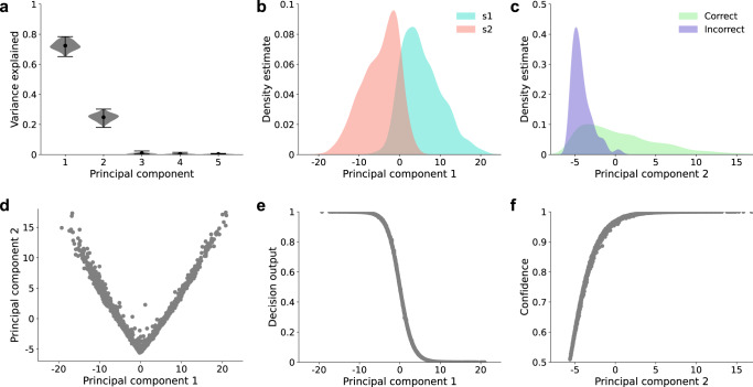
Fig. 7 Learned representations extract a common variable for both decisions and confidence. a Principal component analysis revealed that the learned representations in the model’s penultimate layer were almost entirely explained by the top two principal components. a Reflects probability density over 100 trained networks, with the mean represented by circular markers, and maxima/minima represented by the upper/lower line. b–f Depict results from a single trained network for the purposes of illustrating the model’s learned two-dimensional geometry, but this general representational scheme was shared by all networks. b Kernel density estimates show that the distributions for s1 vs. s2 were separated along PC1. c The distributions for correct vs. incorrect trials were separated along PC2. d PC2 closely resembled a rectification of PC1. e PC1 predicted the model’s decisions. f PC2 predicted the model’s confidence ratings. Note that (d–f) depict trial-by-trial data points, not the predictions of a regression model. Source data are provided as a Source Data file.
Fig. 7 Learned representations extract a common variable for both decisions and confidence. a Principal component analysis revealed that the learned representations in the model’s penultimate layer were almost entirely explained by the top two principal components. a Reflects probability density over 100 trained networks, with the mean represented by circular markers, and maxima/minima represented by the upper/lower line. b–f Depict results from a single trained network for the purposes of illustrating the model’s learned two-dimensional geometry, but this general representational scheme was shared by all networks. b Kernel density estimates show that the distributions for s1 vs. s2 were separated along PC1. c The distributions for correct vs. incorrect trials were separated along PC2. d PC2 closely resembled a rectification of PC1. e PC1 predicted the model’s decisions. f PC2 predicted the model’s confidence ratings. Note that (d–f) depict trial-by-trial data points, not the predictions of a regression model. Source data are provided as a Source Data file.CC BY · PubMed Central
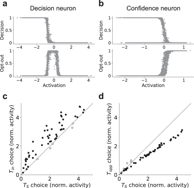
Fig. 8 Analysis of single unit representations. a Example decision neuron, strongly predictive of decision output (Rdecision²=0.83), but not opt-out response (Ropt−out²=0.004). b Example confidence neuron, strongly predictive of opt-out response (Ropt−out²=0.87), but not decision output (Rdecision²=0.16). Kiani & Shadlen3 found that decision-making neurons in the lateral intraparietal cortex (LIP) implicitly coded for confidence. Decision neurons in our neural network model showed this same pattern. c They showed higher activity for trials on which their preferred stimulus (Tin) was chosen vs. trials on which a sure target (TS) was chosen, whereas (d) they were less active for trials on which their non-preferred stimulus (Topp) was chosen. Each point in c and d represents the average normalized (against the pre-stimulus baseline) activation of an individual neuron (over N ≥ 2700 trials) ± the standard error of the mean. Black dots represent neurons with statistically significant deviations from the diagonal (two-sided two-sample t-tests, p < 0.05). White dots represent neurons with non-significant deviations (two-sided two-sample t-tests, p > 0.05). Note that error bars are present on these plots, but are too small to be visible. Neural network results reflect a single example network, but all 100 trained networks displayed a qualitatively similar pattern. Source data are provided as a Source Data file.
Fig. 8 Analysis of single unit representations. a Example decision neuron, strongly predictive of decision output (Rdecision²=0.83), but not opt-out response (Ropt−out²=0.004). b Example confidence neuron, strongly predictive of opt-out response (Ropt−out²=0.87), but not decision output (Rdecision²=0.16). Kiani & Shadlen3 found that decision-making neurons in the lateral intraparietal cortex (LIP) implicitly coded for confidence. Decision neurons in our neural network model showed this same pattern. c They showed higher activity for trials on which their preferred stimulus (Tin) was chosen vs. trials on which a sure target (TS) was chosen, whereas (d) they were less active for trials on which their non-preferred stimulus (Topp) was chosen. Each point in c and d represents the average normalized (against the pre-stimulus baseline) activation of an individual neuron (over N ≥ 2700 trials) ± the standard error of the mean. Black dots represent neurons with statistically significant deviations from the diagonal (two-sided two-sample t-tests, p < 0.05). White dots represent neurons with non-significant deviations (two-sided two-sample t-tests, p > 0.05). Note that error bars are present on these plots, but are too small to be visible. Neural network results reflect a single example network, but all 100 trained networks displayed a qualitatively similar pattern. Source data are provided as a Source Data file.CC BY · PubMed Central
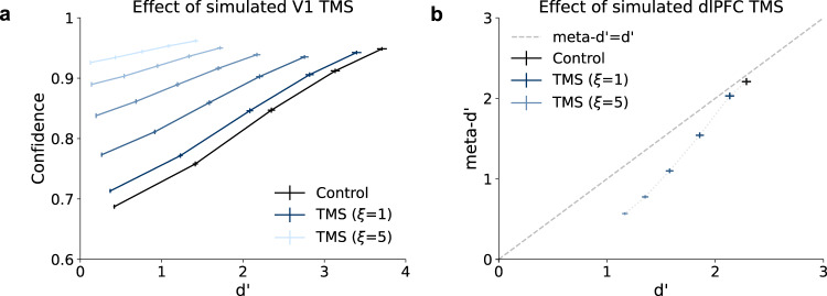
Fig. 9 Simulating TMS to visual and prefrontal cortices. TMS was simulated by adding noise with variance ξ to activations in a specific layer. a Simulated TMS to the first layer of the network resulted in both decreased type-1 sensitivity (d') and increased confidence, as has been observed following TMS to primary visual cortex (V1). b Simulated TMS to the penultimate layer of the network resulted in a selective impairment of type-2 sensitivity (meta-d'), as has been observed following TMS to dorsolateral prefrontal cortex (dlPFC). See Supplementary Fig. S16 for a detection-theoretic explanation of this effect. Source data are provided as a Source Data file.
Fig. 9 Simulating TMS to visual and prefrontal cortices. TMS was simulated by adding noise with variance ξ to activations in a specific layer. a Simulated TMS to the first layer of the network resulted in both decreased type-1 sensitivity (d') and increased confidence, as has been observed following TMS to primary visual cortex (V1). b Simulated TMS to the penultimate layer of the network resulted in a selective impairment of type-2 sensitivity (meta-d'), as has been observed following TMS to dorsolateral prefrontal cortex (dlPFC). See Supplementary Fig. S16 for a detection-theoretic explanation of this effect. Source data are provided as a Source Data file.CC BY · PubMed Central
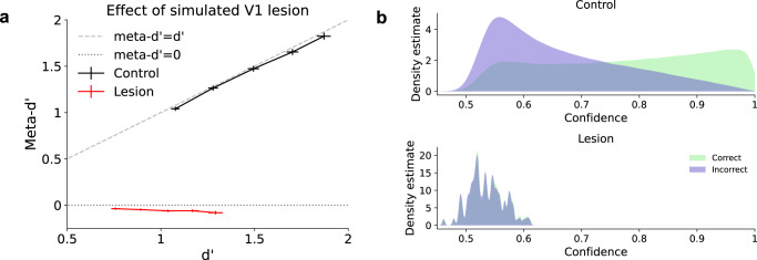
Fig. 10 Simulating blindsight. Lesions to V1 can cause the condition known as blindsight, in which patients have the subjective sensation of blindness despite preserved visual capacity. This pattern can be formalized as a combination of preserved type-1 sensitivity (d'), low visual confidence, and low type-2 sensitivity (meta-d'). a Lesions to V1 were simulated in the model by scaling activations in the first layer of the trained network by a factor of 0.01. This resulted in a sharp reduction in meta-d' despite relatively preserved d'. b Confidence ratings were significantly lower following simulated lesions, and the distribution of confidence ratings showed a nearly complete overlap for correct and incorrect trials, consistent with meta-d' ≈ 0. All results reflect an average over 100 trained networks ± the standard error of the mean. Source data are provided as a Source Data file.
Fig. 10 Simulating blindsight. Lesions to V1 can cause the condition known as blindsight, in which patients have the subjective sensation of blindness despite preserved visual capacity. This pattern can be formalized as a combination of preserved type-1 sensitivity (d'), low visual confidence, and low type-2 sensitivity (meta-d'). a Lesions to V1 were simulated in the model by scaling activations in the first layer of the trained network by a factor of 0.01. This resulted in a sharp reduction in meta-d' despite relatively preserved d'. b Confidence ratings were significantly lower following simulated lesions, and the distribution of confidence ratings showed a nearly complete overlap for correct and incorrect trials, consistent with meta-d' ≈ 0. All results reflect an average over 100 trained networks ± the standard error of the mean. Source data are provided as a Source Data file.CC BY · PubMed Central

Verification

Claims the paper makes

The claims and statistics of this paper haven’t been checked yet.

Run the check — free, no account needed. It reads the open-access text and checks the sources it cites.

A few free checks a day · papers already verified open instantly · results are public

Claims other papers make about this one

Each is checked against this paper’s own text: does it say what the citing paper says it does?

Self-check

Percentages, sums and reported differences re-computed from the paper’s own numbers.

The self-check needs the paper’s full text.

Citations

Cites

Show all 70 references

Research works printed but not linked: 1

  1. Benjamin, A. S. & Bjork, R. A. In Implicit memory and metacognition, 321–350 (Psychology Press, 2014).

Cited by

Sorted by citations

Metadata

Authors
Webb, T. W., Miyoshi, K., So, T. Y., Rajananda, S., & Lau, H.
Affiliations
  • University of California, Los Angeles (US)
  • Kyoto University (JP)
  • University of Hong Kong (HK)
  • Harvard University (US)
  • RIKEN Center for Brain Science (JP)
Corresponding author
  • Webb, Taylor W.
  • Lau, Hakwan
Venue
Nature Communications
Published
2023-07-06
Volume
14
Issue
1
Pages
3992-3992
ISSN
2041-1723 (ISSN-L)
OpenAlex
W4383371132
Cited by
31
References
70
Citations by year
2026: 6 · 2025: 8 · 2024: 7 · 2023: 7
FWCI
4.19
Type
journal article
Language
en
Open access
Locations
  • Nature Communications (publishedVersion, cc-by)
  • bioRxiv (Cold Spring Harbor Laboratory) (acceptedVersion, cc-by)
  • PubMed Central (publishedVersion, cc-by)
  • PubMed (publishedVersion)
  • RePEc: Research Papers in Economics (submittedVersion)
  • DOAJ (DOAJ: Directory of Open Access Journals) (submittedVersion, cc-by-sa)
Funders
U.S. Department of Health & Human Services | NIH | National Institute of Mental Health (F32MH117972)
Topics
  • Life Sciences › Neuroscience › Cognitive Neuroscience › Visual perception and processing mechanisms
  • Social Sciences › Decision Sciences › General Decision Sciences › Decision-Making and Behavioral Economics
  • Life Sciences › Neuroscience › Cognitive Neuroscience › Neural and Behavioral Psychology Studies
Keywords
decision confidence, rational decision-making, naturalistic stimuli, deep neural network, decision variables
MeSH terms
Cognition, Decision Making, Probability, Bias

About these checks

Registry, retraction, Cites and statistics results are computed, not judged, with one exception: a printed reference that no index lists is read once by a model before it counts as a citation error. Claims are extracted by a model and kept only when their quote appears verbatim in the text; each cited source is then checked, with a model’s help, for whether it says what the claim relies on. Those verdicts can be wrong — read the claim’s quote and the cited source before relying on one.

Statistics and arithmetic are recomputed, not judged.

Confidence bands are shown only for fields calibrated on our annotated test set. None is calibrated yet, so no band is shown.

What counts as a claim ›How we measure confidence ›How we check this ›

Are you an author, or do you see a problem with this page? Request a review