

The DOI matches its Crossref record; 68 of the 68 references it cites were found in a registry or an index.
Analysis of microbial compositions: a review of normalization and differential abundance analysis
Open accessAbstract
Increasingly, researchers are discovering associations between microbiome and a wide range of human diseases such as obesity, inflammatory bowel diseases, HIV, and so on. The first step towards microbiome wide association studies is the characterization of the composition of human microbiome under different conditions. Determination of differentially abundant microbes between two or more environments, known as differential abundance (DA) analysis, is a challenging and an important problem that has received considerable interest during the past decade. It is well documented in the literature that the observed microbiome data (OTU/SV table) are relative abundances with an excess of zeros. Since relative abundances sum to a constant, these data are necessarily compositional. In this article we review some recent methods for DA analysis and describe their strengths and weaknesses.
Overview
The claims and statistics of this paper haven’t been checked yet.
Run the check — free, no account needed. It reads the open-access text and checks the sources it cites.
Integrity signals
Registry
Cites
Statistics
Figures
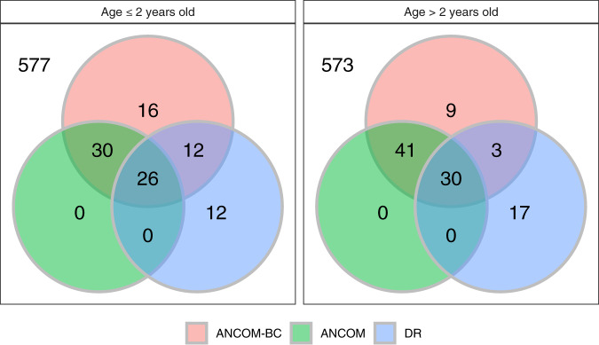
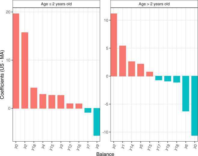
Verification
Claims the paper makes
The claims and statistics of this paper haven’t been checked yet.
Run the check — free, no account needed. It reads the open-access text and checks the sources it cites.
Claims other papers make about this one
Each is checked against this paper’s own text: does it say what the citing paper says it does?
In the citing paper
“A recent approach called differential ranking is robust to the choice of the alr reference feature, and ranks produced from relative abundances are identical to the ranks of absolute abundances66,67.”
From Longitudinal gut microbiome changes in immune checkpoint blockade-treated advanced melanoma (2024) · cites this paper as [66]
Self-check
Percentages, sums and reported differences re-computed from the paper’s own numbers.
The self-check needs the paper’s full text.
Citations
Cites
Controlling the False Discovery Rate: A Practical and Powerful Approach to Multiple Testing
Benjamini, Y., & Hochberg, Y. (1995) · Journal of the Royal Statistical Society Series B: Statistical Methodology · doi:10.1111/j.2517-6161.1995.tb02031.x · Cited by 109,482 · cited 2×
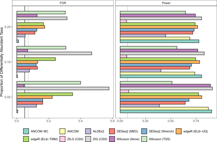
“By default, ANCOM-BC implements Holm-Bonferroni 70 method and other DA methods implement BH procedure 57 to adjust for multiple comparisons.”
MethodModerated estimation of fold change and dispersion for RNA-seq data with DESeq2
Love, M. I., Huber, W., & Anders, S. (2014) · Genome Biology · doi:10.1186/s13059-014-0550-8 · Cited by 95,106 · cited 3×
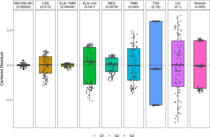
“Some commonly used normalization methods include Cumulative-Sum Scaling (CSS) implemented in metagenome-Seq 21 , Median (MED) in DESeq2 41 , Upper Quartile (UQ) 42 and Trimmed Mean of M-values (TMM) 43 in edgeR 44 and Wrench 45 , and Total-Sum Scaling (TSS) which simply transforms the abundance…”
InfluentialRobinson, M. D., McCarthy, D. J., & Smyth, G. K. (2010) · Bioinformatics · doi:10.1093/bioinformatics/btp616 · Cited by 41,364
DADA2: High–resolution sample inference from Illumina amplicon data
Callahan, B. J., McMurdie, P. J., Rosen, M. J., Han, A. W., Johnson, A. J. A., & Holmes, S. P. (2016) · Nature Methods · doi:10.1038/nmeth.3869 · Cited by 35,698
Reproducible, interactive, scalable and extensible microbiome data science using QIIME 2
Bolyen, E., Rideout, J. R., Dillon, M. R., Bokulich, N. A., Abnet, C. C., Al-Ghalith, G. A., Alexander, H., Alm, E. J., Arumugam, M., Asnicar, F., et al. (2019) · Nature Biotechnology · doi:10.1038/s41587-019-0209-9 · Cited by 23,742
A Simple Sequentially Rejective Multiple Test Procedure
(1979) · Scandinavian Journal of Statistics · doi:10.2307/4615733 · Cited by 21,526 · cited 1×
“The sample sizes in the two age categories (≤2 years, >2 years) for Malawi (MA), USA (US) and Venezuela (VEN) are (47, 36), (50, 260), and (27, 70), respectively.”
BackgroundUPARSE: highly accurate OTU sequences from microbial amplicon reads
Edgar, R. C. (2013) · Nature Methods · doi:10.1038/nmeth.2604 · Cited by 16,770
Metagenomic biomarker discovery and explanation
Segata, N., Izard, J., Waldron, L., Gevers, D., Miropolsky, L., Garrett, W. S., & Huttenhower, C. (2011) · Genome Biology · doi:10.1186/gb-2011-12-6-r60 · Cited by 16,192
Differential expression analysis for sequence count data
Anders, S., & Huber, W. (2010) · Genome Biology · doi:10.1186/gb-2010-11-10-r106 · Cited by 15,581
A scaling normalization method for differential expression analysis of RNA-seq data
Robinson, M. D., & Oshlack, A. (2010) · Genome Biology · doi:10.1186/gb-2010-11-3-r25 · Cited by 7,876
Research works printed but not linked: 1
- Gotelli, N. J. & Colwell, R. K. Estimating species richness. Biol. Divers. Front. Meas. Assess. 12, 39–54 (2011).
Cited by
Sorted by citations
Items 201–300 of 345
RSim: A reference-based normalization method via rank similarity
Yuan, B., & Wang, S. (2023) · PLoS Computational Biology · doi:10.1371/journal.pcbi.1011447 · Cited by 4
Hein, D., Coughlin, L. A., Poulides, N. A., Koh, A. Y., & Sanford, N. N. (2024) · Journal of Immunotherapy and Precision Oncology · doi:10.36401/jipo-23-30 · Cited by 2
Selwyn, J. D., Despard, B. A., Galvan-Dubois, K. A., Trytten, E. C., & Vollmer, S. V. (2025) · Frontiers in Marine Science · doi:10.3389/fmars.2025.1491476 · Cited by 3
“…popular analysis software ANCOM in using the geometric mean of all taxa as the reference rather than one designated reference taxa and also improves the incorporation of 0 data to avoid the use of pseudo-counts which can bias results (Mandal et al., 2015; Kaul et al., 2017; Lin and Peddada, 2020b).”
CODARFE: Unlocking the prediction of continuous environmental variables based on microbiome
Barbosa, M. C., da Silva, J. F. M., Alves, L. C., Finn, R. D., & Paschoal, A. R. (2025) · GigaScience · doi:10.1093/gigascience/giaf055 · Cited by 2
Soil protists in tropical systems: From morphological variation to trophic groups
Schulz, G. (2022) · doi:10.53846/goediss-9126 · Cited by 2
An overview of systematic evidence on oral microbial composition for orodigestive tract cancer risk
Kuriakose, S., Vinutha, R. S., & Shridhar, K. (2022) · Annals of Oncology Research and Therapy · doi:10.4103/aort.aort_11_22 · Cited by 1
Frozen Green Leaves as Potential Nutrient Subsidies in North American Mangrove Ecosystems
Overstreet, K. R., Dangremond, E. M., & Feller, I. C. (2024) · Estuaries and Coasts · doi:10.1007/s12237-024-01457-1 · Cited by 1
“…gradients resulting from seasonal changes (Fer-nandes et al. 2014; Wang et al. 2022) — with a number of studies suggesting that microbial richness and diversity may increase with warmer summer temperatures and decrease with colder winter temperatures (Lin and Das Peddada 2020; Wang et al. 2022).”
Group-wise normalization in differential abundance analysis of microbiome samples
Clark‐Boucher, D., Coull, B. A., Reeder, H. T., Wang, F., Sun, Q., Starr, J. R., & Lee, K. H. (2025) · BMC Bioinformatics · doi:10.1186/s12859-025-06235-9 · Cited by 1
“Ideally, under sparsity assumptions about the proportion of taxa that are differentially abundant, the normalization factors are proportional to the unknown sampling fractions, enabling inference on the absolute abundance scale [19].”
Metzler-Zebeli, B. U., Lerch, F., Yosi, F., Vötterl, J. C., Koger, S., & Klinsoda, J. (2024) · Scientific Reports · doi:10.1038/s41598-024-81227-y · Cited by 1
Instrumental variable estimation for compositional treatments
Ailer, E., Müller, C. L., & Kilbertus, N. (2025) · Scientific Reports · doi:10.1038/s41598-025-89204-9 · Cited by 8
“Since the logarithm is undefined for zero entries, a simple strategy is to add a small constant to all absolute counts, so called pseudo-counts 61,62 .”
Burden, E., Seyoum, Y., Evans, J. P., Thomas, W. J., Kitson, J., Batten, T., Patel, R. C., van der Giezen, M., & Smith, C. (2025) · Journal of Shoulder and Elbow Surgery · doi:10.1016/j.jse.2025.01.044 · Cited by 1
Hernández‐Perea, F. E., Aguirre‐von‐Wobeser, E., Coronado, Y., & de la Torre, M. M. (2025) · Grass and Forage Science · doi:10.1111/gfs.12723 · Cited by 1
Lawless, C., Kovacs, K., Dehcheshmeh, M. M., Ebrahimie, E., Messele, Y. E., Snowball, M., Trott, D. J., & McLelland, D. J. (2025) · Animals · doi:10.3390/ani15131831 · Cited by 1
“Due to the common non-normal distribution of microbial abundance data, high variability, the presence of outliers, zero inflation, and skewness, the median is preferred over the mean as a measure of central tendency in microbiome studies [17,18].”
Logotheti, M., Γκέκας, Θ., Agioutantis, P. C., Hatzimanolis, A., Foteli, S., Mamma, D., Stefanis, N. C., Kolisis, F. N., & Loutrari, H. V. (2025) · Microorganisms · doi:10.3390/microorganisms13081935 · Cited by 1
“Differential abundance analysis was conducted using ANCOM-BC (Analysis of Com-positions of Microbiomes with Bias Correction) [54] in R, enabling the identification of taxa exhibiting significant differences in abundance between groups [55].”
The Gut Microbiota of Peruvian Children Under the Age of Two During the Complementary Feeding Period
Kutbi, A., Gong, J., Dluzen, D. F., Pop, M., & Li, Y. (2025) · International Journal of Environmental Research and Public Health · doi:10.3390/ijerph22091369 · Cited by 1
“For each sample, relative abundance was calculated for each taxon as the proportion of total sequences assigned to that taxon [65].”
Basset, C., & Zaldo-Aubanell, Q. (2025) · Soil Security · doi:10.1016/j.soisec.2025.100203 · Cited by 1
Lipowska, M. M., Sadowska, E. T., Kohl, K. D., & Koteja, P. (2025) · ISME Communications · doi:10.1093/ismeco/ycaf160 · Cited by 3
“The analyses were performed for relative abundances (using adonis2 function), and for the “abso-lute” abundances, using the method of Analysis of Compositions of Microbiome with Bias Correction (ANCOM-BC; ancombc2 function in R package ANCOMBC, v. 2.4.0; [64, 65]).”
InfluentialMeta-Analysis of the Gut Microbiome: An African American Representation
Anushka, K. C., & Paudel, R. (2025) · International Journal of Environmental Research and Public Health · doi:10.3390/ijerph22101591 · Cited by 1
“One method of DAA is the Analysis of Compositions of Microbiomes with Bias Correction (ANCOM-BC) [23].”
InfluentialGut microbial community structure of the adult citrus root weevil Diaprepes abbreviatus
Rodriguez‐Fernandez, I. A., Santiago-Rodríguez, T. M., Figueroa-Pratts, P. G., Cintrón-Berríos, K., Rodriguez-Cornier, N. D., & Toranzos, G. A. (2025) · Frontiers in Insect Science · doi:10.3389/finsc.2025.1676003 · Cited by 1
Coexistence rules for small, antagonistically interacting microbial communities
Athreya, G. S., Gokhale, C. S., & Verma, P. (2025) · PLoS Computational Biology · doi:10.1371/journal.pcbi.1013763 · Cited by 1
“The choice of relative vs absolute densities in empirical data depends on the biological question, e.g. as in the context of microbiome studies [74–76].”
Wu, Q., Lu, S., Wang, L., Liao, X., & Wei, D. (2025) · Gut Pathogens · doi:10.1186/s13099-025-00784-3 · Cited by 1
“Extreme values of 0% and 100% were replaced with 0.001% and 99.999%, respectively [27].”
InfluentialVirulence evolution of a salmonid virus following a host jump
Loeher, M. M., Kurath, G., Kennedy, D. A., Salzer, J. E., Batts, W. N., Breyta, R. B., & Wargo, A. R. (2025) · PLoS Pathogens · doi:10.1371/journal.ppat.1013806 · Cited by 1
Schloss, P. D. (2026) · mSystems · doi:10.1128/msystems.00930-26 · Cited by 1
“…of each OTU in the sample (21, 22); (vi) One CLR, which calculated the CLR after adding a pseudocount of 1 to the abundance of all of the OTUs (21, 22); (vii) the DESeq2 R package (v.1.34.0), which was used to implement the variance stabilizing transformation to normalize the OTU counts (8,…”
InfluentialZheng, K., Qian, B., Liu, T., Wang, B., Xiao, X., Zhou, B., & Huang, R. (2026) · Environmental Technology & Innovation · doi:10.1016/j.eti.2026.104815 · Cited by 1
Lee, E. M., McNulty, N. P., Hibberd, M. C., Cheng, J., Ahsan, K., Chang, H.-W., Cohen, B. A., & Gordon, J. I. (2026) · Nature Communications · doi:10.1038/s41467-026-71871-5 · Cited by 3
Xue, J., Li, M., Chen, W., Pan, L., Zhang, C., Tan, L., Tang, Q., & Tang, D. (2026) · Beverage Plant Research · doi:10.48130/bpr-0025-0046 · Cited by 1
Yang, G., & Jin, G. (2026) · Applied Soil Ecology · doi:10.1016/j.apsoil.2026.107085 · Cited by 1
Best practices framework for using 16S rRNA gene sequencing in poultry microbiota research
Lyte, J. M., Seyoum, M. M., Ayala, D., Kers, J. G., Caputi, V., Johnson, T. J., Zhang, L., Rehberger, J. M., Zhang, G., Dridi, S., et al. (2026) · Poultry Science · doi:10.1016/j.psj.2026.107275 · Cited by 2
“Rarefying is achieved by subsampling to a smaller, predetermined count, typically the fewest sequence read count among the samples, while CSS adjusts counts based on the cumulative sum (Lin and Peddada, 2020b).”
Molina, L., van Dillewijn, P., Velando, F., Hurtado, I., & Segura, A. (2026) · Journal of Environmental Sciences · doi:10.1016/j.jes.2026.105597 · Cited by 1
Reduced Carbon Emissions and Chain Elongation during Mixotrophic Fermentation of a Biomass Feedstock
Afzal, M. X., Bonatelli, M. L., Kleinsteuber, S., Sträuber, H., & Baleeiro, F. C. F. (2026) · ACS Omega · doi:10.1021/acsomega.6c06316 · Cited by 1
Compositional Analysis of Microbiome Data
Xia, Y., & Sun, J. (2023) · Springer eBooks · doi:10.1007/978-3-031-21391-5_14 · Cited by 1
Differential Abundance Analysis of Microbiome Data
Xia, Y., & Sun, J. (2023) · Springer eBooks · doi:10.1007/978-3-031-21391-5_12 · Cited by 1
Sweet Orange Juice Processing By-Product Extracts: A Caries Management Alternative to Chlorhexidine
Saha, S., Boesch, C., Maycock, J., Wood, S. R., & Do, T. (2023) · Biomolecules · doi:10.3390/biom13111607 · Cited by 1
“The human oral and gut microbiome is a vast and complex community of trillions of microbes, containing approximately 45.6 million genes, which is 2000 times more genes than the human genome [1].”
BackgroundInfluentialPraise, S., Miyazawa, M., Phung, L. D., Nishiyama, M., Kumar, A., & Watanabe, T. (2023) · Environmental Pollution · doi:10.1016/j.envpol.2023.122923 · Cited by 1
Xu, J., Dai, Y., Bai, Y., Ge, X., Fang, X., & Zhao, L. (2024) · Journal of Functional Foods · doi:10.1016/j.jff.2024.106155 · Cited by 1
Kinetics and pathways of sub‐lithic microbial community (hypolithon) development
Bosch, J., Lebre, P. H., Marais, E., Maggs‐Kölling, G., & Cowan, D. A. (2024) · Environmental Microbiology Reports · doi:10.1111/1758-2229.13290 · Cited by 1
“To understand the compositional development of the hypolithic microbial communities at the genus level, ANCOM-BC was used to identify differentially abundant genera found in quartz rock and marble tile derived samples compared to samples where no hypolithon development was detected.”
MethodInfluentialHembrom, P. S., Deepthi, M., Kannoth, S., Reeja, N., Antony, G., & Grace, T. (2025) · Microbial Pathogenesis · doi:10.1016/j.micpath.2025.107636 · Cited by 1
Bayesian covariate-dependent graph learning with a dual group spike-and-slab prior
Zeng, Z., Li, M., & Vannucci, M. (2025) · Biometrics · doi:10.1093/biomtc/ujaf053 · Cited by 1
“We apply the centered log ratio transformation to normalize the abundance counts (Aitchison, 1982; Gloor et al., 2017; Lin and Peddada, 2020), as commonly done in Gaussian graphical modeling for microbiome data to satisfy the Gaussian assumption (Kurtz et al., 2015; Wilms and Bien, 2022).”
Tanaka, Y., Bianchi, M. R., & Ismail, N. S. (2023) · Turkish journal of Dental Hygiene · doi:10.51847/w79fik2fuq · Cited by 1
Quiles, K., Shao, F., Johnson, W. E., & Chen, F. F. (2026) · Scientific Reports · doi:10.1038/s41598-025-34926-z · Cited by 1
“…within a host tissue instead, as these values can be more functionally relevant to predict dysbiosis and disease progression over time; parametric models like DESeq2 uses negative binomial distributions applied to normalized data to minimize hidden confounding factors from sample fractions 63 .”
Silva, A. M. M., Feiler, H. P., Lacerda-Júnior, G. V., Fernandes‐Júnior, P. I., Aidar, S. T., de Araújo, V. L. V. P., Matteoli, F. P., Pereira, A. P. A., de Melo, I. S., & Cardoso, E. J. B. N. (2022) · Research Square · doi:10.21203/rs.3.rs-2066211/v1 · Cited by 1
Arbuscular mycorrhizal fungi and rhizobacteria attenuating drought stress in maize plants
Silva, A. M. M. (2023) · doi:10.11606/t.11.2023.tde-03082023-081931 · Cited by 1
Kumar, M., & Field, M. A. (2025) · bioRxiv (Cold Spring Harbor Laboratory) · doi:10.1101/2025.11.03.686403 · Cited by 1
Development of contractor's proposal process model in design-build procurement
Then, D. C. K. (2005)
The Impact Of Dietary Advanced Glycation Endproducts
Linkens, A. M. A. (2022) · Research Publications (Maastricht University) · doi:10.26481/dis.20221005al
Byers, A. K. (2022) · doi:10.5194/egusphere-2022-689-ac1
Byers, A. K. (2022) · doi:10.5194/egusphere-2022-689-ac2
Unravelling the Environmental Variance of Litter Size Through the Genome and Gut Microbiome
Casto‐Rebollo, C. (2023) · RiuNet (Universitat Politècnica de València) · doi:10.4995/thesis/10251/192460
Ferreira, S. C. M., Jarquín‐Díaz, V. H., & Heitlinger, E. G. (2023) · Research Square · doi:10.21203/rs.3.rs-2733243/v1
Dynamics of the microbiome in pancreatic cancer from inception to invasion
Pfisterer, N. (2023) · eDiss (Georg-August-Universität Göttingen) · doi:10.53846/goediss-10152
The gut microbiome-linked long chain fatty acid stearate suppresses colorectal cancerPreprint
Tsenkova, M., Brauer, M., Pozdeev, V. I., Kasakin, M. F., Busi, S. B., Schmoetten, M., Cheung, D., Meyers, M., Rodriguez, F., Gaigneaux, A., et al. (2023) · bioRxiv (Cold Spring Harbor Laboratory) · doi:10.1101/2023.12.07.570549
Maskawa, R., Hideki Takayasu, C., Islam, T., Takayasu, L., Kurokawa, R., Masuoka, H., Suda, W., & Takayasu, M. (2024) · bioRxiv (Cold Spring Harbor Laboratory) · doi:10.1101/2024.03.15.585153
Additional file 4 of Controlling taxa abundance improves metatranscriptomics differential analysis
Ji, Z., & Ma, L. (2023) · Figshare · doi:10.6084/m9.figshare.22618396
Subrata, S. A., Yuda, P., Artama, W. T., Garine-Wichatitsky, M. D., André, A., & MICHAUX, J. R. (2024) · International Microbiology · doi:10.1007/s10123-024-00521-x
“…the magnitude of data variation (i.e., average library size; Weiss et al. (2017)), ecological consideration of original microbiota (McKnight et al. 2019), the importance of phylogenetic tree in the analysis (Liu et al. 2020), and the importance of taxa abundance in the study (Lin and Das 2020).”
mbDecoda: a debiased approach to compositional data analysis for microbiome surveys
Zong, Y., Zhao, H., & Wang, T. (2024) · Briefings in Bioinformatics · doi:10.1093/bib/bbae205
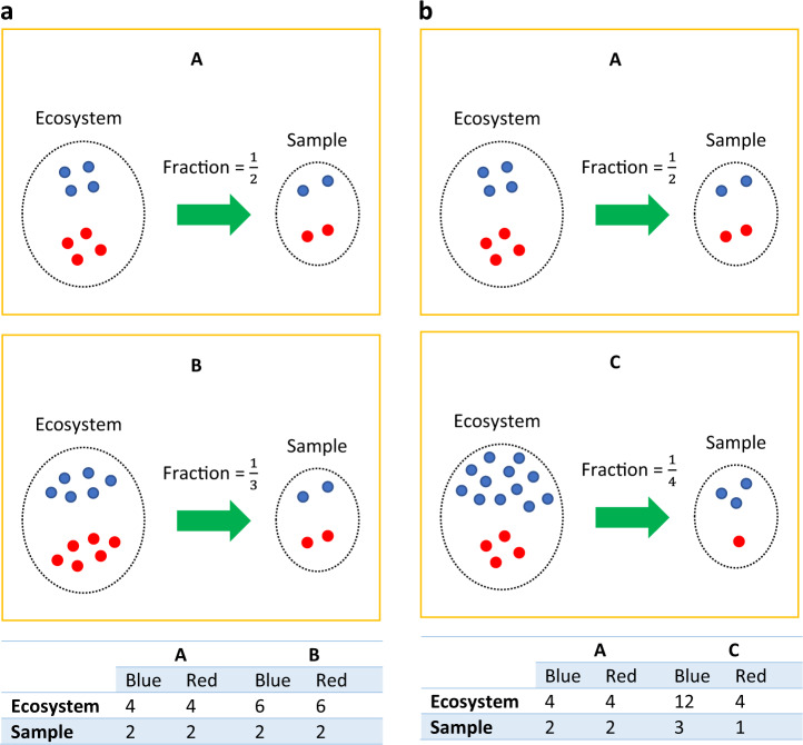
“…contrast to sequencing depth, which represents the amount of sequencing data generated for a single sample, sampling depth, also known as sampling fraction, is defined as the ratio of sequencing depth to total microbial load, assuming an equal probability of sequencing any microbial cell [11, 12].”
BackgroundLipowska, M. M., Sadowska, E. T., Kohl, K. D., & Koteja, P. (2024) · Research Square · doi:10.21203/rs.3.rs-4765186/v1
Taxanorm: a novel taxa-specific normalization approach for microbiome data
Wang, Z., Lloyd, D., Zhao, S., & Motsinger‐Reif, A. A. (2024) · BMC Bioinformatics · doi:10.1186/s12859-024-05918-z
“To handle the zeros commonly seen in microbiome data [15], an arbitrary pseudo count is typically used to replace zeros, but the choice of this arbitrary value can influence downstream analysis [25– 27].”
MethodgLinDA: Global Differential Abundance Analysis of MicrobiomesPreprint
Fehse, L., Tajabadi, M., Martin, R., Holzmann, H., & Heider, D. (2024) · bioRxiv (Cold Spring Harbor Laboratory) · doi:10.1101/2024.09.29.615668
“If a peer’s dataset is too small, the outcome lacks statistical power and tends to show an increased false discovery rate (Lin and Peddada, 2020; Zhou et al., 2022).”
BackgroundGlück, M., Bossdorf, O., & Thomassen, H. A. (2024) · F1000Research · doi:10.12688/f1000research.157160.1
Sample Article for Pree Reviewer
Kumar, V. (2024) · Cobot · doi:10.12688/cobot.17707.1
Belaouni, H. A., Stevenson, M., Rosell, S., & McClure, A. (2024) · bioRxiv (Cold Spring Harbor Laboratory) · doi:10.1101/2024.12.25.630314
Association Between Oral Microbiota and Close-Range Proximity in a Primary SchoolPreprint
Dall’Amico, L., Bai, X., Weltzien, S. M., Rayner, S., Paolotti, D., Budin‐Ljøsne, I., Matussek, A., Furberg, A., Cattuto, C., & Nielsen, C. S. (2024) · bioRxiv (Cold Spring Harbor Laboratory) · doi:10.1101/2024.12.27.628096
“Microbial composition was pro-filed using 16S rRNA gene sequencing, yielding relative abundance distributions for each taxon [35], recorded at the amplicon sequence variant (ASV) resolution.”
Confounder-free Predictive Models for Microbiome-based Host Phenotype PredictionPreprint
Monshizadeh, M., Hong, Y., & Ye, Y. (2025) · bioRxiv (Cold Spring Harbor Laboratory) · doi:10.1101/2025.01.29.635502
CircoTax: a novel circular representation of differentially abundant microbial ranksPreprint
Gloria, L. D., Casbarra, L., & Ramazzotti, M. (2025) · Research Square · doi:10.21203/rs.3.rs-6002535/v1
M’Bra, P. E. H., Avino, M., Lim, E. N. K., Mayhue, M., Balthazar, P., Aumont, A., Prévost, K., Massé, É., & Fernandes, K. J. L. (2025) · bioRxiv (Cold Spring Harbor Laboratory) · doi:10.1101/2025.02.25.640129
Microbiome Experimentation 2.0
Ramanathan, J. (2025) · Springer eBooks · doi:10.1007/978-3-031-80029-0_8
Exploring the Potential of Large Language Models in Differential Abundance AnalysisPreprint
Franco-Alba, R., Goryanin, I. V., & Goryanin, I. (2025) · bioRxiv · doi:10.1101/2025.06.04.657820
“…that are differentially abundant across various conditions or environments, providing insights that are pivotal for understanding microbial communities and their functions, and allowing researchers to identify microbes that are statistically different between two or more conditions [8, 37, 30, 20].”
MITScan : Score-Based Genome-Wide Association Analysis of the Microbiome and Host TranscriptomePreprint
Hao, Y., Kafri, T., & Zou, F. (2025) · bioRxiv (Cold Spring Harbor Laboratory) · doi:10.1101/2025.06.24.661342
Fehse, L., Tajabadi, M., Martin, R., Holzmann, H., & Heider, D. (2025) · Computational and Structural Biotechnology Journal · doi:10.1016/j.csbj.2025.07.031
Guzman, J. P. M. D., Mwamburi, S. M., Lurkpranee, S., Koiwai, K., Kondo, H., & Hırono, I. (2025) · Journal of Fish Diseases · doi:10.1111/jfd.70043
Sieve, A. C., Giuliano, E. A., McAdams, Z. L., Vientós‐Plotts, A. I., Reinero, C. R., & Ericsson, A. C. (2025) · Veterinary Ophthalmology · doi:10.1111/vop.70064
Identification of microbiome markers for ordered groups
Yu, J., Hosain, M. M., & Park, T. (2025) · Genes & Genomics · doi:10.1007/s13258-025-01673-4
Mwamburi, S. M., Guzman, J. P. M. D., Konishi, K., Nozaki, R., Hattori, N., Koiwai, K., Hırono, I., & Kondo, H. (2025) · Fisheries Science · doi:10.1007/s12562-025-01925-y
Root Microbial Functions and Robust Network Drive High-Yielding Canola Genotype
Li, Y., Mamet, S. D., Vail, S. L., & Siciliano, S. D. (2025) · Phytobiomes Journal · doi:10.1094/pbiomes-05-25-0033-r
Smilde, A. K., Marini, F., Westerhuis, J. A., & Liland, K. H. (2025) · doi:10.1002/9781394211241.ref
Metagenomics: Concepts and scope
Tyagi, S., Kanchan, S., Kesheri, M., & Katara, P. (2025) · Elsevier eBooks · doi:10.1016/b978-0-443-21980-1.00004-8
Pig feed as a source of bacterial DNA and its potential impact on porcine gut microbiota studies
Hartinger, K., Lerch, F., Yosi, F., Vötterl, J. C., & Metzler-Zebeli, B. U. (2025) · Frontiers in Animal Science · doi:10.3389/fanim.2025.1710910
Progresses in microbial taxonomy research methods
Bhattacharya, S. (2025) · Proceedings of the Indian National Science Academy · doi:10.1007/s43538-025-00658-x
Trytten, E. C., Despard, B. A., Selwyn, J. D., & Vollmer, S. V. (2025) · ISME Communications · doi:10.1093/ismeco/ycaf247
“This normalization method shows similar performance to the frequently used ANCOM-BC normalization method while also allowing for full contrasts and post hoc tests within modeling frameworks [69], such as the linear mixed-effects models with interactions and post hoc analyses employed here.”
Ferreira, S. C. M., Jarquín‐Díaz, V. H., & Heitlinger, E. G. (2024) · Figshare · doi:10.6084/m9.figshare.26598020
Wang, C., Segal, L. N., Hu, J., Zhou, B., Hayes, R. B., Ahn, J., & Li, H. (2022) · Figshare · doi:10.6084/m9.figshare.20444181
Aya, V., Jiménez, P., Muñoz, E., & Ramírez, J. D. (2024) · Figshare · doi:10.6084/m9.figshare.26596778
Additional file 2 of Controlling taxa abundance improves metatranscriptomics differential analysis
Ji, Z., & Ma, L. (2023) · Figshare · doi:10.6084/m9.figshare.22618390
Ferreira, S. C. M., Jarquín‐Díaz, V. H., & Heitlinger, E. G. (2024) · Figshare · doi:10.6084/m9.figshare.26598023
Ferreira, S. C. M., Jarquín‐Díaz, V. H., & Heitlinger, E. G. (2024) · Figshare · doi:10.6084/m9.figshare.26598014
Coffey, E. L., Gomez, A. M., Ericsson, A. C., Burton, E. N., Granick, J. L., Lulıch, J. P., & Furrow, E. (2023) · Figshare · doi:10.6084/m9.figshare.22631463
Ferreira, S. C. M., Jarquín‐Díaz, V. H., & Heitlinger, E. G. (2024) · Figshare · doi:10.6084/m9.figshare.26598026
Additional file 1 of Relative abundance data can misrepresent heritability of the microbiome
Bruijning, M., Ayroles, J. F., Henry, L. P., Koskella, B., Meyer, K., & Metcalf, C. J. E. (2023) · Figshare · doi:10.6084/m9.figshare.24277149
Coffey, E. L., Gomez, A. M., Ericsson, A. C., Burton, E. N., Granick, J. L., Lulıch, J. P., & Furrow, E. (2023) · Figshare · doi:10.6084/m9.figshare.22631460
Ferreira, S. C. M., Jarquín‐Díaz, V. H., & Heitlinger, E. G. (2024) · Figshare · doi:10.6084/m9.figshare.26598017
Additional file 1 of Controlling taxa abundance improves metatranscriptomics differential analysis
Ji, Z., & Ma, L. (2023) · Figshare · doi:10.6084/m9.figshare.22618387
Additional file 1 of Taxanorm: a novel taxa-specific normalization approach for microbiome data
Wang, Z., Lloyd, D., Zhao, S., & Motsinger‐Reif, A. A. (2024) · Figshare · doi:10.6084/m9.figshare.27042494
Coffey, E. L., Gomez, A. M., Ericsson, A. C., Burton, E. N., Granick, J. L., Lulıch, J. P., & Furrow, E. (2023) · Figshare · doi:10.6084/m9.figshare.22631448
Coffey, E. L., Gomez, A. M., Ericsson, A. C., Burton, E. N., Granick, J. L., Lulıch, J. P., & Furrow, E. (2023) · Figshare · doi:10.6084/m9.figshare.22631451
Coffey, E. L., Gomez, A. M., Ericsson, A. C., Burton, E. N., Granick, J. L., Lulıch, J. P., & Furrow, E. (2023) · Figshare · doi:10.6084/m9.figshare.22631457
Metadata
- Authors
- Lin, H., & Peddada, S. D.
- Affiliations
- National Institutes of Health (US)
- Corresponding author
- Peddada, Shyamal Das
- Venue
- npj Biofilms and Microbiomes
- Published
- 2020-12-02
- Volume
- 6
- Issue
- 1
- Pages
- 60-60
- ISSN
- 2055-5008 (ISSN-L)
- PMC
- PMC7710733
- OpenAlex
- W3109541743
- Cited by
- 341
- References
- 68
- Citations by year
- 2026: 57 · 2025: 73 · 2024: 67 · 2023: 77 · 2022: 55 · 2021: 11
- FWCI
- 3.45
- Type
- journal article
- Language
- en
- Open access
- gold
- doi.org
- Locations
- npj Biofilms and Microbiomes (publishedVersion, cc-by)
- PubMed Central (publishedVersion, cc-by)
- PubMed (publishedVersion)
- Funders
- University of Pittsburgh
- Topics
- Life Sciences › Biochemistry, Genetics and Molecular Biology › Molecular Biology › Gut microbiota and health
- Physical Sciences › Environmental Science › Ecology › Microbial Community Ecology and Physiology
- Life Sciences › Biochemistry, Genetics and Molecular Biology › Molecular Biology › Genomics and Phylogenetic Studies
- Keywords
- microbiome, differential abundance, compositional data, normalization, zero-inflated data, OTU table, sequencing read counts, human microbiome
- MeSH terms
- Gastrointestinal Microbiome, Bacteria, Humans, Models, Theoretical, Mouth, Phylogeny
About these checks
Registry, retraction, Cites and statistics results are computed, not judged, with one exception: a printed reference that no index lists is read once by a model before it counts as a citation error. Claims are extracted by a model and kept only when their quote appears verbatim in the text; each cited source is then checked, with a model’s help, for whether it says what the claim relies on. Those verdicts can be wrong — read the claim’s quote and the cited source before relying on one.
Statistics and arithmetic are recomputed, not judged.
Confidence bands are shown only for fields calibrated on our annotated test set. None is calibrated yet, so no band is shown.
What counts as a claim ›How we measure confidence ›How we check this ›
Are you an author, or do you see a problem with this page? Request a review
