

The DOI matches its Crossref record; 54 of the 54 references it cites were found in a registry or an index; 2 of the 2 sources its claims cite were checked for support.
Learning the natural history of human disease with generative transformers
Open accessAbstract
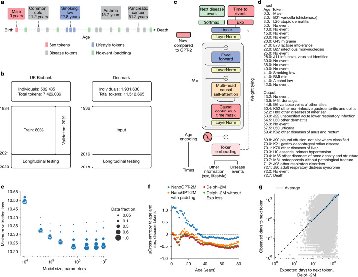
Decision-making in healthcare relies on understanding patients’ past and current health states to predict and, ultimately, change their future course 1–3 . Artificial intelligence (AI) methods promise to aid this task by learning patterns of disease progression from large corpora of health records 4,5 . However, their potential has not been fully investigated at scale. Here we modify the GPT 6 (generative pretrained transformer) architecture to model the progression and competing nature of human diseases. We train this model, Delphi-2M, on data from 0.4 million UK Biobank participants and validate it using external data from 1.9 million Danish individuals with no change in parameters. Delphi-2M predicts the rates of more than 1,000 diseases, conditional on each individual’s past disease history, with accuracy comparable to that of existing single-disease models. Delphi-2M’s generative nature also enables sampling of synthetic future health trajectories, providing meaningful estimates of potential disease burden for up to 20 years, and enabling the training of AI models that have never seen actual data. Explainable AI methods 7 provide insights into Delphi-2M’s predictions, revealing clusters of co-morbidities within and across disease chapters and their time-dependent consequences on future health, but also highlight biases learnt from training data. In summary, transformer-based models appear to be well suited for predictive and generative health-related tasks, are applicable to population-scale datasets and provide insights into temporal dependencies between disease events, potentially improving the understanding of personalized health risks and informing precision medicine approaches.
Overview
AI snapshot
Written from the paper’s full text.
TL;DR
Delphi-2M adapts GPT-2 to model continuous-time disease trajectories and predicts rates for more than 1,000 ICD-10 diagnoses conditional on past health history. Trained on UK Biobank and externally tested on Danish registries, it matches or exceeds many single-disease models and can generate synthetic future health trajectories.
Key findings
- Delphi-2M was trained on 402,799 UK Biobank participants (80%) and validated on 100,639 (20%), with external testing on 1.93 million Danish individuals; it predicts 1,256 disease tokens plus death.
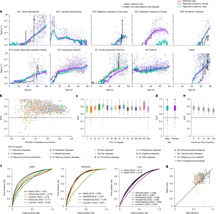
- Internal validation average age-stratified AUC was approximately 0.76, with death at 0.97; performance decreased to an average of 0.70 after 10 years. External Danish testing gave average AUC 0.67 (s.d. 0.09) versus UK Biobank longitudinal testing 0.69 (s.d. 0.09), with disease-level correlation 0.76 (95% CI 0.72–0.80).
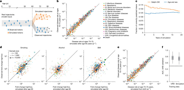
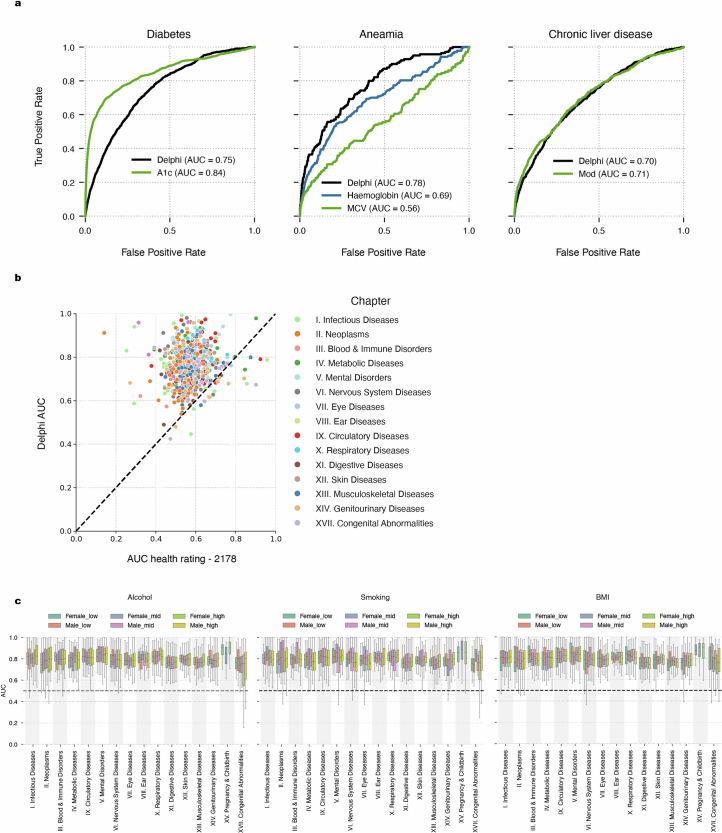
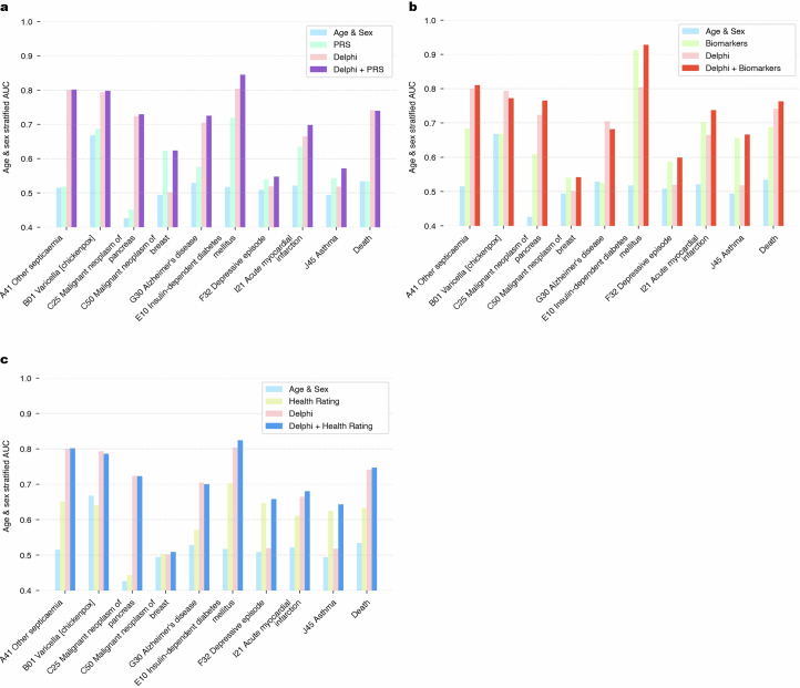
- Generative sampling from age 60 reproduced future incidence at ages 70–75; 17% of disease tokens were correctly predicted in the first year, dropping to less than 14% after 20 years, compared with 12–13% using sex and age alone. A model trained only on synthetic data achieved average AUC 0.74, three percentage points lower than the original.
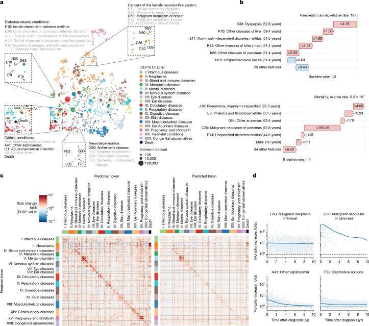
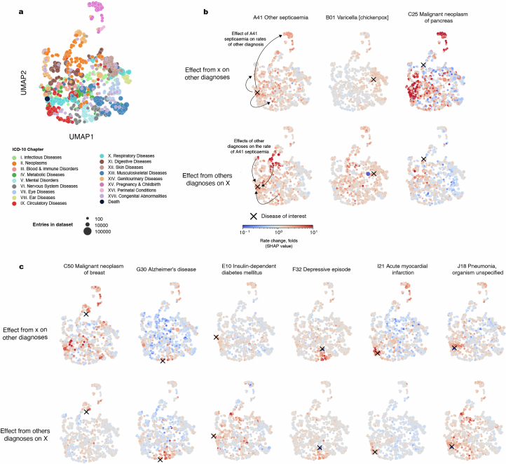
- SHAP analyses showed digestive-tract diagnoses elevated pancreatic cancer risk 19-fold, and pancreatic cancer increased mortality rate almost ten thousandfold; cancer effects on mortality decayed over several years, whereas septicaemia effects were short-lived.
Methods
- Design: modified GPT-2 architecture with continuous age encoding using sine/cosine functions, an added exponential waiting-time output head, and causal attention masks that also mask same-time tokens; trained with Adam for 200,000 iterations.
- Data: UK Biobank first-occurrence ICD-10 level 3 diagnoses, cancer registry data, sex, BMI, smoking, alcohol, and death; Danish National Patient Registry and Causes of Death registry for external validation, restricted to ages 50–80 on 1 January 2016.
- Analysis: age- and sex-stratified AUC, calibration, cross-entropy, longitudinal testing with a 1-year gap, generative trajectory sampling, UMAP of token embeddings, SHAP for token influence, and comparisons with clinical risk scores, biomarker models, and other machine learning methods.
Limitations
- Stated: UK Biobank has healthy volunteer and participant selection biases, including immortal time bias before recruitment; missingness across self-report, primary care, hospital, cancer, and death sources is learned by the model; limited follow-up beyond age 80 makes that period unreliable; subgroup differences by ancestry and deprivation were observed; and temporal dependencies should not be interpreted as causal.
- Stated: lifestyle token times were randomized by −20 to +40 years from recruitment to break confounding with mortality jumps, which “probably also diminishes the true effect of these tokens.”
- Evident: external Danish validation showed lower average AUC (0.67) than UK Biobank longitudinal testing (0.69), and the paper notes that some learned associations may be artefacts of incomplete aggregated UK Biobank data rather than true diagnostic pathways.
Model-written summary. Check it against the paper before relying on it.
Integrity signals
Registry
Cites
Statistics
Figures
Verification
Claims the paper makes
30 Own result · 13 Own interpretation · 9 No basis given · 7 Own method · 2 Partly supported · 1 Not checked yet · accuracy not yet measured
The cited sources support only part of this claim — read each source’s verdict below.
In the paper
“The UK Biobank comprises more white British citizens than the general population, and the participants tend to be on average more affluent and educated32.”
§ Learning the natural history of human disease with generative transformers > External validation and bias assessment
What the sources say
- Partly supportedcites [32] Fry, A. et al. Comparison of sociodemographic and health-related characteristics of UK Biobank participants with those of the general population. Am. J. Epidemiol. 186, 1026–1034 (2017). sourceExperimental — accuracy not yet measured
The Discussion (page unavailable) says UK Biobank participants generally live in less socioeconomically deprived areas, supporting the claim’s affluence component as an area-level proxy. The paper passages found do not compare participants’ education with that of the general population, so the education component is unsupported. (LLM, conf=0.84)
plaincorrelational- Asserted: passes — The authors put it forward as true.
- Checkable: passes — It can be checked against evidence.
- Load-bearing: unclear — It is unclear whether the paper’s conclusions depend on it.
- Based: passes — The paper gives a reason why it holds.
- Partly supported
The cited sources support only part of this claim — read each source’s verdict below.
In the paper
“The UK Biobank comprises more white British citizens than the general population, and the participants tend to be on average more affluent and educated32.”
§ Learning the natural history of human disease with generative transformers > External validation and bias assessment
What the sources say
- Partly supportedcites [32] Fry, A. et al. Comparison of sociodemographic and health-related characteristics of UK Biobank participants with those of the general population. Am. J. Epidemiol. 186, 1026–1034 (2017). sourceExperimental — accuracy not yet measured
Table 1 in the Results shows a higher proportion of white participants in UK Biobank (94.6%) than in the 2011 census population aged 40–69 (91.3%). But its footnote says the “White” category includes white British, white Irish, and other white backgrounds; the table does not establish a higher proportion specifically of white British people. (LLM, conf=0.85)
plaincorrelational- Asserted: passes — The authors put it forward as true.
- Checkable: passes — It can be checked against evidence.
- Load-bearing: passes — The paper’s conclusions depend on it.
- Based: passes — The paper gives a reason why it holds.
- Partly supported
A result the paper reports from its own data — it cites no other source for it, so there is none to check. The quote shows it is in the paper.
In the paper
“Among the most confidently predicted next events is death, with an age-stratified AUC of 0.97 in both sexes.”
§ Learning the natural history of human disease with generative transformers > Modelling multi-disease incidences
plain- Asserted: passes — The authors put it forward as true.
- Checkable: passes — It can be checked against evidence.
- Load-bearing: unclear — It is unclear whether the paper’s conclusions depend on it.
- Based: passes — The paper gives a reason why it holds.
A result the paper reports from its own data — it cites no other source for it, so there is none to check. The quote shows it is in the paper.
In the paper
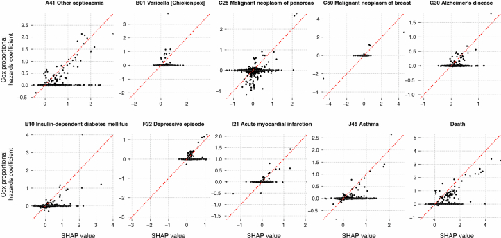
“SHAP analysis of data from 100,639 individuals of the validation cohort reveals the mutual dependencies by which each disease, sex and lifestyle token influences the rate of subsequent disease tokens, similar to hazard ratios in conventional statistical models”
§ Learning the natural history of human disease with generative transformers > Explaining Delphi-2M predictions
plaindirectn = 100,639- Asserted: passes — The authors put it forward as true.
- Checkable: passes — It can be checked against evidence.
- Load-bearing: passes — The paper’s conclusions depend on it.
- Based: passes — The paper gives a reason why it holds.
A result the paper reports from its own data — it cites no other source for it, so there is none to check. The quote shows it is in the paper.
In the paper
“A detailed analysis of UK Biobank’s first occurrence data revealed several biases, reflected by Delphi-2M.”
§ Learning the natural history of human disease with generative transformers > Discussion
plaincorrelational- Asserted: passes — The authors put it forward as true.
- Checkable: passes — It can be checked against evidence.
- Load-bearing: passes — The paper’s conclusions depend on it.
- Based: passes — The paper gives a reason why it holds.
A result the paper reports from its own data — it cites no other source for it, so there is none to check. The quote shows it is in the paper.
In the paper
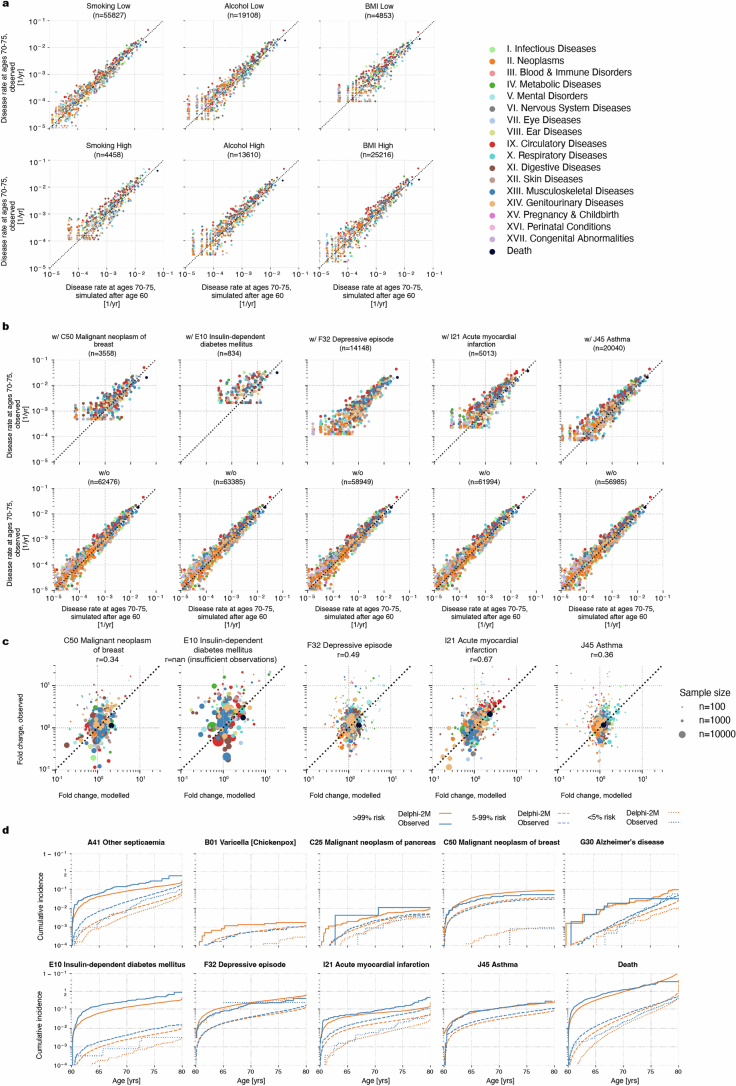
“the disease incidences at ages 70–75 years are well recapitulated, showing that the overall distributions are well preserved by iterative sampling”
§ Learning the natural history of human disease with generative transformers > Sampling future disease trajectories
boosted- Asserted: passes — The authors put it forward as true.
- Checkable: passes — It can be checked against evidence.
- Load-bearing: passes — The paper’s conclusions depend on it.
- Based: passes — The paper gives a reason why it holds.
The paper states this without a source or data behind it here, so there is nothing to check it against. The quote shows it is in the paper.
In the paper
“Septicaemia, for example, is diagnosed in 93% of cases in a hospital setting and is predicted to occur at 8× greater rates in individuals with any other hospital data.”
§ Learning the natural history of human disease with generative transformers > External validation and bias assessment
plain- Asserted: passes — The authors put it forward as true.
- Checkable: passes — It can be checked against evidence.
- Load-bearing: unclear — It is unclear whether the paper’s conclusions depend on it.
- Based: passes — The paper gives a reason why it holds.
A result the paper reports from its own data — it cites no other source for it, so there is none to check. The quote shows it is in the paper.
In the paper
“Delphi-2M’s ability to quantify the temporal influence of previous health data revealed that cancers increase mortality in a sustained manner, while the effects of myocardial infarction or septicaemia regress within 5 years.”
§ Learning the natural history of human disease with generative transformers > Discussion
plaindirect- Asserted: passes — The authors put it forward as true.
- Checkable: passes — It can be checked against evidence.
- Load-bearing: passes — The paper’s conclusions depend on it.
- Based: passes — The paper gives a reason why it holds.
- The authors state this as an assumption: The waiting times from the current event to each competing event are exponentially distributed with rates λi = exp(logitsi).
- The authors state this as an assumption: The rates λi are constant in time over short periods.
A result the paper reports from its own data — it cites no other source for it, so there is none to check. The quote shows it is in the paper.
In the paper
“For 97% of diagnoses, the AUC was greater than 0.5”
§ Learning the natural history of human disease with generative transformers > Modelling multi-disease incidences
plain- Asserted: passes — The authors put it forward as true.
- Checkable: passes — It can be checked against evidence.
- Load-bearing: passes — The paper’s conclusions depend on it.
- Based: passes — The paper gives a reason why it holds.
A result the paper reports from its own data — it cites no other source for it, so there is none to check. The quote shows it is in the paper.
In the paper
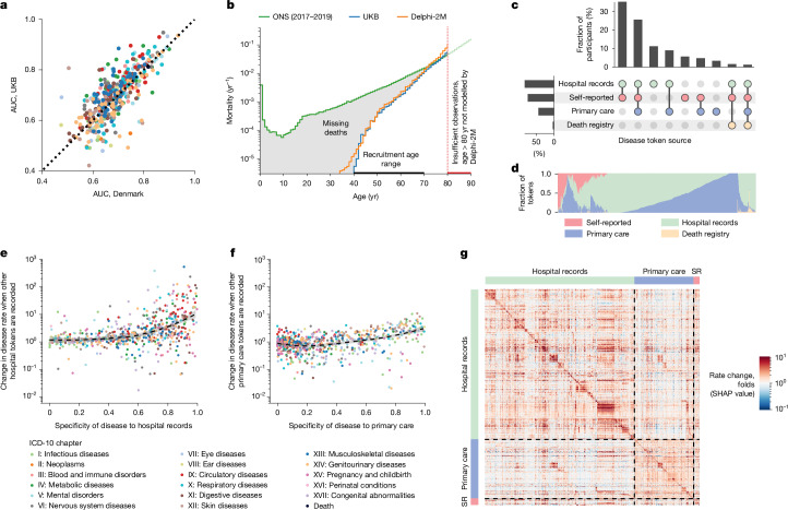
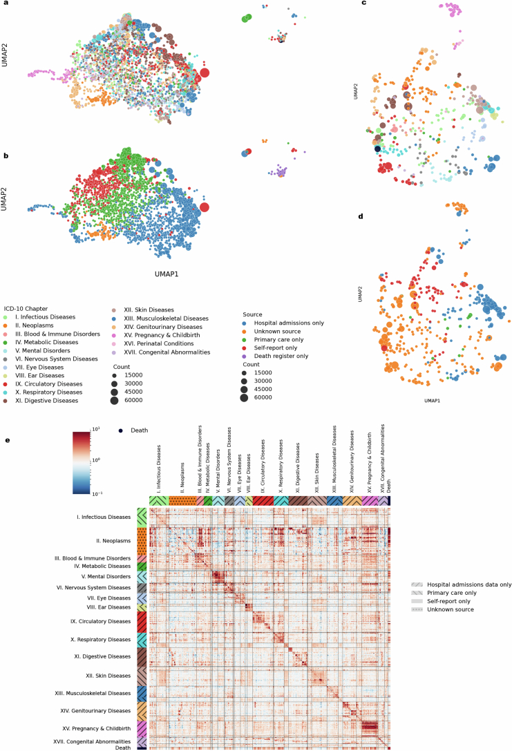
“However, the underlying sources were not always available for each participant and time period (Fig. 5c and Supplementary Fig. 12).”
§ Learning the natural history of human disease with generative transformers > External validation and bias assessment
plain- Asserted: passes — The authors put it forward as true.
- Checkable: passes — It can be checked against evidence.
- Load-bearing: passes — The paper’s conclusions depend on it.
- Based: passes — The paper gives a reason why it holds.
- It may state two separate claims as one. 20
- Probably not a substantial claim. 8
A result the paper reports from its own data — it cites no other source for it, so there is none to check. The quote shows it is in the paper.
In the paper
“self-reporting and GP records contain mostly common diseases, while data from hospital records include more-aggressive disease tokens, such as myocardial infarction or septicaemia (Fig. 5d).”
§ Learning the natural history of human disease with generative transformers > External validation and bias assessment
plaincorrelational- Asserted: passes — The authors put it forward as true.
- Checkable: passes — It can be checked against evidence.
- Load-bearing: passes — The paper’s conclusions depend on it.
- Based: passes — The paper gives a reason why it holds.
It may state two separate claims as one.
A result the paper reports from its own data — it cites no other source for it, so there is none to check. The quote shows it is in the paper.
In the paper
“The average AUC when Delphi-2M is applied to Danish data was 0.67 (s.d. 0.09), which is lower than for longitudinal testing on UKB data (0.69, s.d. 0.09).”
§ Learning the natural history of human disease with generative transformers > External validation and bias assessment
plain- Asserted: passes — The authors put it forward as true.
- Checkable: passes — It can be checked against evidence.
- Load-bearing: passes — The paper’s conclusions depend on it.
- Based: passes — The paper gives a reason why it holds.
It may state two separate claims as one.
None of the sources cited for this claim have been checked yet.
In the paper
“Explainable AI methods7 provide insights into Delphi-2M’s predictions, revealing clusters of co-morbidities within and across disease chapters and their time-dependent consequences on future health, but also highlight biases learnt from training data.”
§ Learning the natural history of human disease with generative transformers > Abstract
plaincorrelational- Asserted: passes — The authors put it forward as true.
- Checkable: passes — It can be checked against evidence.
- Load-bearing: passes — The paper’s conclusions depend on it.
- Based: passes — The paper gives a reason why it holds.
It may state two separate claims as one.
A result the paper reports from its own data — it cites no other source for it, so there is none to check. The quote shows it is in the paper.
In the paper
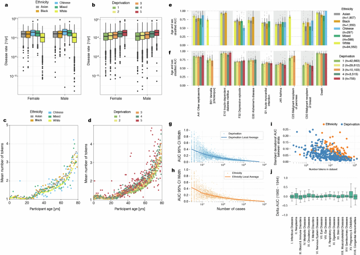
“Lower rates of diseases are reported among participants of white ethnicity, and the rate of diagnoses increases with deprivation—trends that are reproduced by Delphi-2M (Extended Data Fig. 9).”
§ Learning the natural history of human disease with generative transformers > External validation and bias assessment
plaindirect- Asserted: passes — The authors put it forward as true.
- Checkable: passes — It can be checked against evidence.
- Load-bearing: passes — The paper’s conclusions depend on it.
- Based: passes — The paper gives a reason why it holds.
It may state two separate claims as one.
A result the paper reports from its own data — it cites no other source for it, so there is none to check. The quote shows it is in the paper.
In the paper
“Delphi-2M’s ability to quantify the temporal influence of previous health data revealed that cancers increase mortality in a sustained manner, while the effects of myocardial infarction or septicaemia regress within 5 years.”
§ Learning the natural history of human disease with generative transformers > Discussion
plaindirect- Asserted: passes — The authors put it forward as true.
- Checkable: passes — It can be checked against evidence.
- Load-bearing: passes — The paper’s conclusions depend on it.
- Based: passes — The paper gives a reason why it holds.
It may state two separate claims as one.
- The authors state this as an assumption: The waiting times from the current event to each competing event are exponentially distributed with rates λi = exp(logitsi).
- The authors state this as an assumption: The rates λi are constant in time over short periods.
A result the paper reports from its own data — it cites no other source for it, so there is none to check. The quote shows it is in the paper.
In the paper
“We estimated a version with the level 3 codes as well and this did perform marginally worse.”
§ Learning the natural history of human disease with generative transformers > Methods > Model longitudinal evaluation
plain- Asserted: passes — The authors put it forward as true.
- Checkable: passes — It can be checked against evidence.
- Load-bearing: fails — The paper’s conclusions may not depend on it.
- Based: passes — The paper gives a reason why it holds.
Probably not a substantial claim. The paper’s conclusions may not depend on it.
The paper states this without a source or data behind it here, so there is nothing to check it against. The quote shows it is in the paper.
In the paper
“Delphi-2M’s generative nature also enables sampling of synthetic future health trajectories, providing meaningful estimates of potential disease burden for up to 20 years, and enabling the training of AI models that have never seen actual data.”
§ Learning the natural history of human disease with generative transformers > Abstract
plaindirect- Asserted: passes — The authors put it forward as true.
- Checkable: passes — It can be checked against evidence.
- Load-bearing: passes — The paper’s conclusions depend on it.
- Based: passes — The paper gives a reason why it holds.
It may state two separate claims as one.
The paper states this without a source or data behind it here, so there is nothing to check it against. The quote shows it is in the paper.
In the paper
“Note that Delphi’s predictions are generally strongly influenced by statistical chance and compatible with a range of outcomes for a given individual.”
§ Learning the natural history of human disease with generative transformers > Discussion
boostedcorrelational- Asserted: passes — The authors put it forward as true.
- Checkable: passes — It can be checked against evidence.
- Load-bearing: fails — The paper’s conclusions may not depend on it.
- Based: fails — The paper may give no reason why it holds.
Probably not a substantial claim. The paper’s conclusions may not depend on it. The paper may give no reason why it holds. It may state two separate claims as one.
A result the paper reports from its own data — it cites no other source for it, so there is none to check. The quote shows it is in the paper.
In the paper
“In the first year of sampling, there are on average 17% disease tokens that are correctly predicted, and this drops to less than 14% 20 years later. These figures compare to values of 12–13% of correctly predicted disease tokens using sex and age alone”
§ Learning the natural history of human disease with generative transformers > Sampling future disease trajectories
plaincorrelational- Asserted: passes — The authors put it forward as true.
- Checkable: passes — It can be checked against evidence.
- Load-bearing: passes — The paper’s conclusions depend on it.
- Based: passes — The paper gives a reason why it holds.
It may state two separate claims as one.
What the paper did — it cites no source for this, so there is none to check. The quote shows it is in the paper.
In the paper
“Internal longitudinal testing was carried out using data for all individuals still alive by the cut-off date (471,057) and evaluated on incidence from 1 July 2021 to 1 July 2022, therefore enforcing a 1 year data gap between predictions and evaluation.”
§ Learning the natural history of human disease with generative transformers > Methods > Data
plain- Asserted: passes — The authors put it forward as true.
- Checkable: passes — It can be checked against evidence.
- Load-bearing: passes — The paper’s conclusions depend on it.
- Based: passes — The paper gives a reason why it holds.
Probably not a substantial claim. It may state two separate claims as one.
A conclusion the paper draws from its own results — it cites no other source for it, so there is none to check. The quote shows it is in the paper.
In the paper
“This creates a selection bias, as no deaths are recorded before recruitment, which has direct implications for the estimated mortality (Fig. 5b).”
§ Learning the natural history of human disease with generative transformers > External validation and bias assessment
plaindirect- Asserted: passes — The authors put it forward as true.
- Checkable: passes — It can be checked against evidence.
- Load-bearing: passes — The paper’s conclusions depend on it.
- Based: passes — The paper gives a reason why it holds.
It may state two separate claims as one.
A conclusion the paper draws from its own results — it cites no other source for it, so there is none to check. The quote shows it is in the paper.
In the paper
“In addition to a healthy volunteer bias and participant selection bias before recruitment, the diverse nature of health data sources impacted Delphi’s prediction, as UK-Biobank-specific patterns of missingness were exploited to infer disease rates.”
§ Learning the natural history of human disease with generative transformers > Discussion
plaindirect- Asserted: passes — The authors put it forward as true.
- Checkable: passes — It can be checked against evidence.
- Load-bearing: passes — The paper’s conclusions depend on it.
- Based: passes — The paper gives a reason why it holds.
It may state two separate claims as one.
A conclusion the paper draws from its own results — it cites no other source for it, so there is none to check. The quote shows it is in the paper.
In the paper
“In summary, transformer-based models appear to be well suited for predictive and generative health-related tasks, are applicable to population-scale datasets and provide insights into temporal dependencies between disease events”
§ Learning the natural history of human disease with generative transformers > Abstract
hedgedcorrelational- Asserted: passes — The authors put it forward as true.
- Checkable: passes — It can be checked against evidence.
- Load-bearing: passes — The paper’s conclusions depend on it.
- Based: unclear — It is unclear why the paper says it holds.
It may state two separate claims as one.
What the paper did — it cites no source for this, so there is none to check. The quote shows it is in the paper.
In the paper
“We train this model, Delphi-2M, on data from 0.4 million UK Biobank participants and validate it using external data from 1.9 million Danish individuals with no change in parameters.”
§ Learning the natural history of human disease with generative transformers > Abstract
plain- Asserted: passes — The authors put it forward as true.
- Checkable: passes — It can be checked against evidence.
- Load-bearing: passes — The paper’s conclusions depend on it.
- Based: passes — The paper gives a reason why it holds.
It may state two separate claims as one.
What the paper did — it cites no source for this, so there is none to check. The quote shows it is in the paper.
In the paper
“External longitudinal testing was conducted on the Danish registries. All individuals residing in Denmark 50–80 years of age on the 1 January 2016 were included. Predictions are based on the available data up to this point and were subsequently evaluated on incidence from 1 January 2017 to 1 of January 2018, similar to the internal longitudinal testing.”
§ Learning the natural history of human disease with generative transformers > Methods > Data
plain- Asserted: passes — The authors put it forward as true.
- Checkable: passes — It can be checked against evidence.
- Load-bearing: passes — The paper’s conclusions depend on it.
- Based: passes — The paper gives a reason why it holds.
Probably not a substantial claim. It may state two separate claims as one.
A conclusion the paper draws from its own results — it cites no other source for it, so there is none to check. The quote shows it is in the paper.
In the paper
“Delphi-2M is uniquely capable of sampling future disease trajectories, which enables the estimation of cumulative disease burdens over periods of up to 20 years, conditional on previous health information.”
§ Learning the natural history of human disease with generative transformers > Discussion
plaindirect- Asserted: passes — The authors put it forward as true.
- Checkable: passes — It can be checked against evidence.
- Load-bearing: passes — The paper’s conclusions depend on it.
- Based: passes — The paper gives a reason why it holds.
It may state two separate claims as one.
- The authors state this as an assumption: The waiting times from the current event to each competing event are exponentially distributed with rates λi = exp(logitsi).
- The authors state this as an assumption: The rates λi are constant in time over short periods.
The paper states this without a source or data behind it here, so there is nothing to check it against. The quote shows it is in the paper.
In the paper
“Under the null hypothesis, these standardized residuals should follow a standard normal distribution.”
§ Learning the natural history of human disease with generative transformers > Methods > Model evaluation
plain- Asserted: passes — The authors put it forward as true.
- Checkable: passes — It can be checked against evidence.
- Load-bearing: passes — The paper’s conclusions depend on it.
- Based: fails — The paper may give no reason why it holds.
Probably not a substantial claim. The paper may give no reason why it holds.
The paper states this without a source or data behind it here, so there is nothing to check it against. The quote shows it is in the paper.
In the paper
“Under the null hypothesis, this sum follows a χ2 distribution with degrees of freedom equal to (n − 1), where n is the number of subgroups.”
§ Learning the natural history of human disease with generative transformers > Methods > Model evaluation
plain- Asserted: passes — The authors put it forward as true.
- Checkable: passes — It can be checked against evidence.
- Load-bearing: passes — The paper’s conclusions depend on it.
- Based: fails — The paper may give no reason why it holds.
Probably not a substantial claim. The paper may give no reason why it holds.
What the paper did — it cites no source for this, so there is none to check. The quote shows it is in the paper.
In the paper
“Predictions were evaluated on 0.96 million disease tokens across 796 ICD-10 codes (each with at least 25 cases).”
§ Learning the natural history of human disease with generative transformers > Methods > Data
plainn = 25- Asserted: passes — The authors put it forward as true.
- Checkable: passes — It can be checked against evidence.
- Load-bearing: passes — The paper’s conclusions depend on it.
- Based: passes — The paper gives a reason why it holds.
Probably not a substantial claim.
What the paper did — it cites no source for this, so there is none to check. The quote shows it is in the paper.
In the paper
“Reproducibility of the method has been confirmed by retraining Delphi-2M using different train-validation splits (n = 4 independent experiments; Supplementary Fig. 1) and testing the trained model using longitudinal UK Biobank data and external data from the Danish National Patient Registry.”
§ Learning the natural history of human disease with generative transformers > Methods > Statistics and reproducibility
plainn = 4- Asserted: passes — The authors put it forward as true.
- Checkable: passes — It can be checked against evidence.
- Load-bearing: passes — The paper’s conclusions depend on it.
- Based: passes — The paper gives a reason why it holds.
It may state two separate claims as one.
What the paper did — it cites no source for this, so there is none to check. The quote shows it is in the paper.
In the paper
“This has two advantages: (1) we can enforce an explicit cut-off and separate data to avoid any potential time-leakage; and (2) we obtain insights into Delphi-2M prognostic capabilities and generalization.”
§ Learning the natural history of human disease with generative transformers > Methods > Model longitudinal evaluation
plaindirect- Asserted: passes — The authors put it forward as true.
- Checkable: passes — It can be checked against evidence.
- Load-bearing: passes — The paper’s conclusions depend on it.
- Based: passes — The paper gives a reason why it holds.
It may state two separate claims as one.
A conclusion the paper draws from its own results — it cites no other source for it, so there is none to check. The quote shows it is in the paper.
In the paper
“The fact that Delphi-2M can be applied to Danish population data with slightly reduced accuracy indicates that many patterns learned by the model accurately reflect the true evolution of multi-morbidity, while also highlighting the existence of differences within each cohort.”
§ Learning the natural history of human disease with generative transformers > External validation and bias assessment
hedgedcorrelational- Asserted: passes — The authors put it forward as true.
- Checkable: passes — It can be checked against evidence.
- Load-bearing: passes — The paper’s conclusions depend on it.
- Based: passes — The paper gives a reason why it holds.
It may state two separate claims as one.
What the paper did — it cites no source for this, so there is none to check. The quote shows it is in the paper.
In the paper
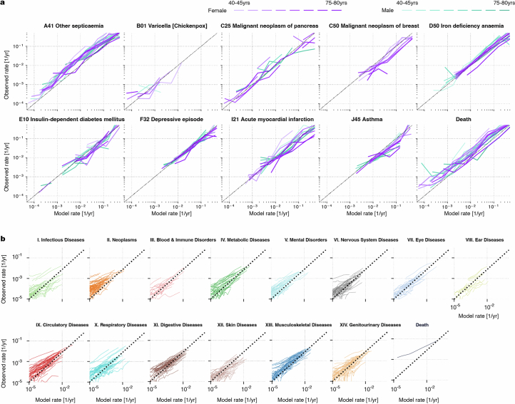
“calibration analyses in 5-year age brackets show that the predicted rates closely match the observed number of cases, showing that the models’ rates of the next tokens are consistently estimated”
§ Learning the natural history of human disease with generative transformers > Modelling multi-disease incidences
plain- Asserted: passes — The authors put it forward as true.
- Checkable: passes — It can be checked against evidence.
- Load-bearing: passes — The paper’s conclusions depend on it.
- Based: passes — The paper gives a reason why it holds.
It may state two separate claims as one.
A conclusion the paper draws from its own results — it cites no other source for it, so there is none to check. The quote shows it is in the paper.
In the paper
“Furthermore, limited follow-up data are currently available for individuals 80 years of age and older. This period is therefore not reliably modelled by Delphi-2M.”
§ Learning the natural history of human disease with generative transformers > External validation and bias assessment
plaindirect- Asserted: passes — The authors put it forward as true.
- Checkable: passes — It can be checked against evidence.
- Load-bearing: unclear — It is unclear whether the paper’s conclusions depend on it.
- Based: passes — The paper gives a reason why it holds.
It may state two separate claims as one.
The paper states this without a source or data behind it here, so there is nothing to check it against. The quote shows it is in the paper.
In the paper
“Under the null hypothesis that all subgroups have the same true AUC (no bias), any observed differences would be attributable to statistical variance.”
§ Learning the natural history of human disease with generative transformers > Methods > Model evaluation
hedged- Asserted: passes — The authors put it forward as true.
- Checkable: passes — It can be checked against evidence.
- Load-bearing: passes — The paper’s conclusions depend on it.
- Based: fails — The paper may give no reason why it holds.
Probably not a substantial claim. The paper may give no reason why it holds.
The authors state this as an assumption.
A person's health trajectory can be represented by a sequence of diagnoses using top-level ICD-10 codes recorded at the age of first diagnosis as well as death.
“A person’s health trajectory can be represented by a sequence of diagnoses using top-level ICD-10 codes recorded at the age of first diagnosis as well as death.”
The authors state this as an assumption.
Health cannot be understood only by the presentation of individual diagnoses but in the context of an individual's co-morbidities and their evolution over time.
“Critically, health cannot only be understood by the presentation of individual diagnoses but, rather, in the context of an individual’s co-morbidities and their evolution over time.”
The authors state this as an assumption.
The waiting times from the current event to each competing event are exponentially distributed with rates λi = exp(logitsi).
“Assuming the Ti are each exponentially distributed waiting times with rates λi = exp(logitsi), the next event being j is equivalent to Tj being the first of the competing waiting times, that is, Tj = min Ti, or equivalently j = argmin Ti.”
The authors state this as an assumption.
The rates λi are constant in time over short periods.
“These approximations hold as long as the rates λi are constant in time, which is a reasonable assumption over short periods.”
Self-check
Percentages, sums and reported differences re-computed from the paper’s own numbers.
Each contradiction between two passages listed here was confirmed by an independent check.
Rated minor: it would not touch a result — a value no result rests on, a p-value that stays on the same side of the significance level, or a conflict that is clerical, resolved elsewhere in the paper, or outside its own findings.
In the paper
§ Learning the natural history of human disease with generative transformers > Sampling future disease trajectories
“This provides the opportunity to compare 63,662 sampled and observed trajectories.”
§ Learning the natural history of human disease with generative transformers > Sampling future disease trajectories
“Delphi-2M is used to simulate health trajectories using validation data (n = 63,622 individuals with disease records both before and after 60 years of age) observed until the age of 60.”
Citations
Cites
Bray, F., Laversanne, M., Sung, H., Ferlay, J., Siegel, R. L., Soerjomataram, I., & Jemal, A. (2024) · CA: a cancer journal for clinicians · doi:10.3322/caac.21834 · Cited by 27,064
Language Models are Few-Shot Learners
Brown, T. B., Mann, B., Ryder, N., Subbiah, M., Kaplan, J., Dhariwal, P., Neelakantan, A., Shyam, P., Sastry, G., Askell, A., et al. (2020) · arXiv · doi:10.48550/arxiv.2005.14165 · Cited by 23,372
DeLong, E. R., DeLong, D. M., & Clarke-Pearson, D. L. (1988) · Biometrics · doi:10.2307/2531595 · Cited by 22,649
Multiple Imputation for Nonresponse in Surveys
Rubin, D. B. (1987) · Wiley Series in Probability and Statistics · doi:10.1002/9780470316696 · Cited by 20,701
mice: Multivariate Imputation by Chained Equations in R
Buuren, S. V., & Groothuis-Oudshoorn, K. (2011) · Journal of Statistical Software · doi:10.18637/jss.v045.i03 · Cited by 13,870
Sudlow, C., Gallacher, J., Allen, N., Beral, V., Burton, P., Danesh, J., Downey, P., Elliott, P., Green, J., Landray, M., et al. (2015) · PLOS Medicine · doi:10.1371/journal.pmed.1001779 · Cited by 12,728
Comorbidity measures for use with administrative data.
Elixhauser, A., Steiner, C., Harris, D. R., & Coffey, R. M. (1998) · Medical Care · doi:10.1097/00005650-199801000-00004 · Cited by 9,921
UMAP: Uniform Manifold Approximation and Projection
McInnes, L., Healy, J., Saul, N., & Großberger, L. (2018) · Journal of Open Source Software · doi:10.21105/joss.00861 · Cited by 9,826
General Cardiovascular Risk Profile for Use in Primary Care: The Framingham Heart Study
D’Agostino, R. B., Vasan, R. S., Pencina, M. J., Wolf, P. A., Cobain, M., Massaro, J. M., & Kannel, W. B. (2008) · Circulation · doi:10.1161/circulationaha.107.699579 · Cited by 7,491
UMAP: Uniform Manifold Approximation and Projection for Dimension Reduction
McInnes, L., Healy, J., & Melville, J. (2018) · arXiv · doi:10.48550/arxiv.1802.03426 · Cited by 7,101
Quan, H., Li, B., Couris, C. M., Fushimi, K., Graham, P. J., Hider, P., Januel, J., & Sundararajan, V. (2011) · American Journal of Epidemiology · doi:10.1093/aje/kwq433 · Cited by 5,967
Social conditions as fundamental causes of disease.
Link, B. G., & Phelan, J. (1995) · Journal of Health and Social Behavior · doi:10.2307/2626958 · Cited by 5,722
2013 ACC/AHA Guideline on the Assessment of Cardiovascular Risk
Goff, D. C., Lloyd-Jones, D. M., Bennett, G., Coady, S., D’Agostino, R. B., Gibbons, R., Greenland, P., Lackland, D. T., Levy, D., O’Donnell, C. J., et al. (2014) · Journal of the American College of Cardiology · doi:10.1016/j.jacc.2013.11.005 · Cited by 4,945
The Danish National Patient Registry: a review of content, data quality, and research potential
Schmidt, M., Schmidt, S. A. J., Sandegaard, J. L., Ehrenstein, V., Pedersen, L. H., & Sørensen, H. T. (2015) · Clinical Epidemiology · doi:10.2147/clep.s91125 · Cited by 4,832
LLaMA: Open and Efficient Foundation Language Models
Touvron, H., Lavril, T., Izacard, G., Martinet, X., Lachaux, M.-A., Lacroix, T., Rozière, B., Goyal, N., Hambro, E., Azhar, F., et al. (2023) · arXiv · doi:10.48550/arxiv.2302.13971 · Cited by 4,602
Fry, A., Littlejohns, T. J., Sudlow, C., Doherty, N., Adamska, L., Sprosen, T., Collins, R., & Allen, N. E. (2017) · American Journal of Epidemiology · doi:10.1093/aje/kwx246 · Cited by 3,979
Goff, D. C., Lloyd-Jones, D. M., Bennett, G., Coady, S., D’Agostino, R. B., Gibbons, R., Greenland, P., Lackland, D. T., Levy, D., O’Donnell, C. J., et al. (2014) · Circulation · doi:10.1161/01.cir.0000437741.48606.98 · Cited by 3,697
Training Language Models to Follow Instructions with Human Feedback
Ouyang, L., Wu, J., Jiang, X., Almeida, D., Wainwright, C., Mishkin, P., Zhang, C., Agarwal, S., Slama, K., Ray, A., et al. (2022) · Advances in Neural Information Processing Systems 35 · doi:10.52202/068431-2011 · Cited by 3,117
The Danish Register of Causes of Death
Helweg‐Larsen, K. (2011) · Scandinavian Journal of Public Health · doi:10.1177/1403494811399958 · Cited by 1,735
Hippisley-Cox, J., Coupland, C., & Brindle, P. (2017) · BMJ · doi:10.1136/bmj.j2099 · Cited by 1,703
Nonparametric Inference for a Family of Counting Processes
Aalen, O. O. (1978) · The Annals of Statistics · doi:10.1214/aos/1176344247 · Cited by 1,505
Development and validation of the American Heart Association’s PREVENT equations
Khan, S. S., Matsushita, K., Sang, Y., Ballew, S. H., Grams, M. E., Surapaneni, A., Blaha, M. J., Carson, A. P., Chang, A. R., Ciemins, E., et al. (2024) · Circulation · doi:10.1161/circulationaha.123.067626 · Cited by 1,234
Gemini: A Family of Highly Capable Multimodal Models
Gemini Team, Anil, R., Borgeaud, S., Alayrac, J.-B., Yu, J., Soricut, R., Schalkwyk, J., Dai, A. M., Hauth, A., Millican, K., et al. (2023) · arXiv · doi:10.48550/arxiv.2312.11805 · Cited by 990
Causal associations between risk factors and common diseases inferred from GWAS summary data
Zhu, Z., Zheng, Z., Zhang, F., Wu, Y., Trzaskowski, M., Maier, R., Robinson, M. R., McGrath, J. J., Visscher, P. M., Wray, N. R., et al. (2018) · Nature Communications · doi:10.1038/s41467-017-02317-2 · Cited by 951
Training Compute-Optimal Large Language Models
Hoffmann, J., Borgeaud, S., Mensch, A., Buchatskaya, E., Cai, T., Rutherford, E., Casas, D. D. L., Hendricks, L. A., Welbl, J., Clark, A., et al. (2022) · Advances in Neural Information Processing Systems 35 · doi:10.52202/068431-2176 · Cited by 932
Rasmy, L., Xiang, Y., Xie, Z., Tao, C., & Zhi, D. (2021) · npj Digital Medicine · doi:10.1038/s41746-021-00455-y · Cited by 886
McClelland, R. L., Jorgensen, N. W., Budoff, M. J., Blaha, M. J., Post, W. S., Kronmal, R. A., Bild, D. E., Shea, S., Liu, K., Watson, K. E., et al. (2015) · Journal of the American College of Cardiology · doi:10.1016/j.jacc.2015.08.035 · Cited by 685
BEHRT: Transformer for Electronic Health Records
Li, Y., Rao, S., Solares, J. R. A., Hassaine, A., Ramakrishnan, R., Canoy, D., Zhu, Y., Rahimi, K., & Salimi-Khorshidi, G. (2020) · Scientific Reports · doi:10.1038/s41598-020-62922-y · Cited by 595
Retrieval Augmentation Reduces Hallucination in Conversation
Shuster, K., Poff, S., Chen, M., Kiela, D., & Weston, J. (2021) · Findings of the Association for Computational Linguistics: EMNLP 2021 · doi:10.18653/v1/2021.findings-emnlp.320 · Cited by 575
Theory and Applications of Hazard Plotting for Censored Failure Data
Nelson, W. B. (1972) · Technometrics · doi:10.1080/00401706.1972.10488991 · Cited by 526
Grattafiori, A., Dubey, A., Jauhri, A., Pandey, A., Kadian, A., Al-Dahle, A., Letman, A., Mathur, A., Schelten, A., Vaughan, A., et al. (2024) · arXiv · doi:10.48550/arxiv.2407.21783 · Cited by 505
A deep learning algorithm to predict risk of pancreatic cancer from disease trajectories
Placido, D., Yuan, B., Hjaltelin, J. X., Zheng, C., Haue, A. D., Chmura, P. J., Yuan, C., Kim, J., Umeton, R., Antell, G., et al. (2023) · Nature Medicine · doi:10.1038/s41591-023-02332-5 · Cited by 349
Self-citationAssociation of Healthy Lifestyle With Years Lived Without Major Chronic Diseases
Nyberg, S. T., Singh‐Manoux, A., Pentti, J., Madsen, I. E. H., Sabia, S., Alfredsson, L. S., Bjørner, J. B., Borritz, M., Burr, H., Goldberg, M., et al. (2020) · JAMA Internal Medicine · doi:10.1001/jamainternmed.2020.0618 · Cited by 308
Adaptation of the Charlson Comorbidity Index for Register-Based Research in Sweden
Ludvigsson, J. F., Appelros, P., Askling, J., Byberg, L., Carrero, J. J., Ekström, A. M., Ekström, M. P., Smedby, K. E. E., Hagström, H., James, S. K., et al. (2021) · Clinical Epidemiology · doi:10.2147/clep.s282475 · Cited by 291
Hippisley‐Cox, J., & Coupland, C. A. C. (2015) · BMJ Open · doi:10.1136/bmjopen-2015-007825 · Cited by 177
Kraljevic, Z., Bean, D., Shek, A., Bendayan, R., Hemingway, H., Yeung, J. A., Deng, A., Balston, A., Ross, J., Idowu, E., et al. (2024) · The Lancet Digital Health · doi:10.1016/s2589-7500(24)00025-6 · Cited by 169 · cited 1×
“However, despite promising proof of concepts 24 , the potential for comprehensive and generative modeling of multi-morbidity has not been fully assessed yet.”
Yang, Z., Mitra, A., Liu, W., Berlowitz, D., & Yu, H. (2023) · Nature Communications · doi:10.1038/s41467-023-43715-z · Cited by 158
Li, Y., Mamouei, M., Salimi-Khorshidi, G., Rao, S., Hassaine, A., Canoy, D., Lukasiewicz, T., & Rahimi, K. (2023) · IEEE Journal of Biomedical and Health Informatics · doi:10.1109/jbhi.2022.3224727 · Cited by 156
Garg, M., Karpiński, M., Matelska, D., Middleton, L., Burren, O. S., Hu, F., Wheeler, E., Smith, K. R., Fabre, M. A., Mitchell, J., et al. (2024) · Nature Genetics · doi:10.1038/s41588-024-01898-1 · Cited by 134
Using sequences of life-events to predict human lives
Savcisens, G., Eliassi‐Rad, T., Hansen, L. K., Mortensen, L. H., Lilleholt, L., Rogers, A., Zettler, I., & Lehmann, S. (2023) · Nature Computational Science · doi:10.1038/s43588-023-00573-5 · Cited by 95
Self-citationMatsushita, K., Kaptoge, S. K., Hageman, S. H. J., Sang, Y., Ballew, S. H., Grams, M. E., Surapaneni, A., Sun, L., Ärnlöv, J., Božić, M., et al. (2022) · European Journal of Preventive Cardiology · doi:10.1093/eurjpc/zwac176 · Cited by 84
Imrie, F., Cebere, B., McKinney, E. F., & van der Schaar, M. (2023) · PLOS Digital Health · doi:10.1371/journal.pdig.0000276 · Cited by 53
Risk-Adapted Starting Age of Screening for Relatives of Patients With Breast Cancer
Mukama, T., Kharazmi, E., Xu, X., Sundquist, K., Sundquist, J., Brenner, H., & Fallah, M. (2019) · JAMA Oncology · doi:10.1001/jamaoncol.2019.3876 · Cited by 49
Development and validation of a dementia risk score in the UK Biobank and Whitehall II cohorts
Anatürk, M., Patel, R., Ebmeier, K. P., Georgiopoulos, G. A., Newby, D., Topiwala, A., de Lange, A. G., Cole, J. H., Jansen, M. G., Singh‐Manoux, A., et al. (2023) · BMJ Mental Health · doi:10.1136/bmjment-2023-300719 · Cited by 49
Tian, Y., Kharazmi, E., Brenner, H., Xu, X., Sundquist, K., Sundquist, J., & Fallah, M. (2020) · Gastroenterology · doi:10.1053/j.gastro.2020.03.063 · Cited by 43
Advancing Multimodal Medical Capabilities of Gemini
Yang, L., Xu, S., Sellergren, A., Kohlberger, T., Zhou, Y., Ktena, I., Kiraly, A., Ahmed, F., Hormozdiari, F., Jaroensri, T., et al. (2024) · arXiv · doi:10.48550/arxiv.2405.03162 · Cited by 34
A unidirectional mapping of ICD-8 to ICD-10 codes, for harmonized longitudinal analysis of diseases
Pedersen, M. K., Eriksson, R., Reguant, R., Collin, C. B., Pedersen, H., Sørup, F. K. H., Simon, C., Birch, A. M., Larsen, M., Nielsen, A. P., et al. (2023) · European Journal of Epidemiology · doi:10.1007/s10654-023-01027-y · Cited by 22
Self-citationRedefining digital health interfaces with large language models
Imrie, F., Rauba, P., & van der Schaar, M. (2025) · Frontiers in Artificial Intelligence · doi:10.3389/frai.2025.1623339 · Cited by 11
RiskScorescvd: Cardiovascular Risk Scores Calculator
Perez-Vicencio, D., Doudesis, D., Thurston, A. J. F., & Selva, J. J. (2023) · doi:10.32614/cran.package.riskscorescvd · Cited by 7
Large Language Models for Medical Forecasting -- Foresight 2Preprint
Kraljević, Ž., Yeung, J. A., Bean, D. M., Teo, J., & Dobson, R. (2024) · arXiv (Cornell University) · doi:10.48550/arxiv.2412.10848 · Cited by 7
Bayesian Cox regression for large-scale inference with applications to electronic health records
Jung, A. W., & Gerstung, M. (2023) · The Annals of Applied Statistics · doi:10.1214/22-aoas1658 · Cited by 4
Self-citationpreventr: An Implementation of the PREVENT and Pooled Cohort Equations
Mayer, M. G. (2024) · doi:10.32614/cran.package.preventr · Cited by 4
OpenAI, Achiam, J., Adler, S., Agarwal, S., Ahmad, L., Akkaya, I., Aleman, F. L., Almeida, D., Altenschmidt, J., Altman, S., et al. (2023) · arXiv · doi:10.48550/arxiv.2303.08774
Redefining Digital Health Interfaces with Large Language Models
Imrie, F., Rauba, P., & van der Schaar, M. (2023) · arXiv · doi:10.48550/arxiv.2310.03560
Research works printed but not linked: 3
- Lundberg, S. M. & Lee, S.-I. A unified approach to interpreting model predictions. Adv. Neural Inf. Process. Syst. 30, 4768–4777 (2017).
- Vaswani, A. et al. Attention is all you need. Adv. Neural Inf. Process. Syst. 30, 6000–6010 (2017).
- Steinberg, E., Fries, J. A., Xu, Y. & Shah, N. H. MOTOR: a time-to-event foundation model for structured medical records. Int. Conf. Learn. Represent. https://iclr.cc/virtual/2024/poster/18777 (2024)
Cited by
Sorted by citations
Chen, H., Shi, Y., Yuan, M., Li, H., & Liu, X. (2025) · Biotechnology Advances · doi:10.1016/j.biotechadv.2025.108785 · Cited by 18
Artificial Intelligence for Cardiovascular Care in Action
Biswas, D., Thangaraj, P., Pedroso, A. F., Ogunniyi, M. O., Maddox, T. M., Ahmad, F. S., & Khera, R. (2025) · JACC Advances · doi:10.1016/j.jacadv.2025.102307 · Cited by 16
Do we actually need aging clocks?
Kriukov, D. V., Efimov, E., Gelfand, M. S., Moskalev, A., & Khrameeva, E. E. (2025) · npj Aging · doi:10.1038/s41514-025-00312-2 · Cited by 13
Health Galaxy: A Multi-organ Trajectory-Computing Framework in Type 2 Diabetes
Lv, H., Li, J., Li, D., Sheng, B., & Wang, Z. (2026) · Research · doi:10.34133/research.1378 · Cited by 11
Neuroimmune Dysregulation and AI-Driven Therapeutic Strategies in Alzheimer’s Disease
Ghosh, S., Bhaskar, R., Singh, D. K. K., Sharma, S., Yarlagadda, B., Sinha, J. K., & Han, S. S. (2025) · Cellular and Molecular Neurobiology · doi:10.1007/s10571-025-01651-0 · Cited by 11
Metadata
- Authors
- Shmatko, A., Jung, A. W., Gaurav, K., Brunak, S., Mortensen, L. H., Birney, E., Fitzgerald, T., & Gerstung, M.
- Affiliations
- European Bioinformatics Institute (GB)
- University of Copenhagen (DK)
- Corresponding author
- Birney, Ewan
- Gerstung, Moritz
- ORCID
- Venue
- Nature
- Published
- 2025-09-17
- Volume
- 647
- Issue
- 8088
- Pages
- 248-256
- ISSN
- 0028-0836 (ISSN-L)
- 1476-4687
- PMC
- PMC12589094
- OpenAlex
- W4414274945
- Semantic Scholar
- d480376f7b315aba50e4b214b4bd545b6d63fefb
- Cited by
- 110
- References
- 42
- Citations by year
- 2026: 92 · 2025: 18
- FWCI
- 43.84
- Type
- journal article
- Language
- en
- Update notices
- correction (2025-11-12)
- Open access
- hybrid
- doi.org
- Locations
- Nature (publishedVersion, cc-by)
- PubMed (publishedVersion)
- Research at the University of Copenhagen (University of Copenhagen) (publishedVersion, cc-by)
- Europe PMC (PubMed Central) (submittedVersion, cc-by)
- Funders
- Deutsches Krebsforschungszentrum
- Topics
- Physical Sciences › Computer Science › Artificial Intelligence › Machine Learning in Healthcare
- Health Sciences › Medicine › Health Informatics › Artificial Intelligence in Healthcare and Education
- Health Sciences › Health Professions › Health Information Management › Artificial Intelligence in Healthcare
- Keywords
- disease progression prediction, generative pre-trained transformer, UK Biobank, explainable AI, precision medicine
- MeSH terms
- Artificial Intelligence, Denmark, Disease, Female, Humans, Male, Comorbidity, Biological Specimen Banks, Disease Progression
About these checks
Registry, retraction, Cites and statistics results are computed, not judged, with one exception: a printed reference that no index lists is read once by a model before it counts as a citation error. Claims are extracted by a model and kept only when their quote appears verbatim in the text; each cited source is then checked, with a model’s help, for whether it says what the claim relies on. Those verdicts can be wrong — read the claim’s quote and the cited source before relying on one.
A language model drew the claims from the paper on 2026-10-27, under version 3 of the claim definition (model deepseek-v4.1-flash, prompt extract-v3).
A second model labelled each claim on 2026-10-27 (model jev-1.13-20260917, definition revision gold-guideline-v0.2).
Cited sources are checked with a language model’s help (gpt-6-sol).
Statistics and arithmetic are recomputed, not judged.
Confidence bands are shown only for fields calibrated on our annotated test set. None is calibrated yet, so no band is shown.
What counts as a claim ›How we measure confidence ›How we check this ›
Are you an author, or do you see a problem with this page? Request a review
