Student or educator? Sign up with your school email and get 6 months of Pro free.
Cited by 120CRISPR and Genetic EngineeringSingle-cell and spatial transcriptomicsGene Regulatory Network Analysis

The DOI matches its Crossref record; 93 of the 93 references it cites were found in a registry or an index.

Scalable genetic screening for regulatory circuits using compressed Perturb-seq

Open access

Abstract

Pooled CRISPR screens with single-cell RNA sequencing readout (Perturb-seq) have emerged as a key technique in functional genomics, but they are limited in scale by cost and combinatorial complexity. In this study, we modified the design of Perturb-seq by incorporating algorithms applied to random, low-dimensional observations. Compressed Perturb-seq measures multiple random perturbations per cell or multiple cells per droplet and computationally decompresses these measurements by leveraging the sparse structure of regulatory circuits. Applied to 598 genes in the immune response to bacterial lipopolysaccharide, compressed Perturb-seq achieves the same accuracy as conventional Perturb-seq with an order of magnitude cost reduction and greater power to learn genetic interactions. We identified known and novel regulators of immune responses and uncovered evolutionarily constrained genes with downstream targets enriched for immune disease heritability, including many missed by existing genome-wide association studies. Our framework enables new scales of interrogation for a foundational method in functional genomics.

Overview

The claims and statistics of this paper haven’t been checked yet.

Run the check — free, no account needed. It reads the open-access text and checks the sources it cites.

A few free checks a day · papers already verified open instantly · results are public

Integrity signals

Registry

Crossref · 10.1038/s41587-023-01964-9

Cites

93 of 93 references verified0 citation errors · 0 not checkable

Statistics

Figures

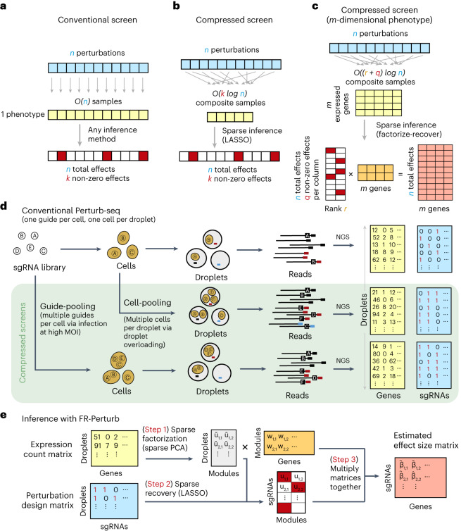
Fig. 1 Framework for compressed Perturb-seq. a, Schematic for conventional perturbation screen with single-valued phenotype. Each sample (yellow) receives a single perturbation (blue). The required number of samples scales linearly with the number of perturbations, as captured by the O(n) term. b, Schematic for compressed perturbation screen with single-valued phenotype. Each ‘composite’ sample (yellow) represents a random combination of perturbations (blue). The required number of samples scales sub-linearly with the number of perturbations given the following: (1) the effects of the perturbations are sparse (that is, k increases more slowly than n), and (2) sparse inference (typically LASSO) is used to infer the effects from the composite sample phenotypes. c, Schematic for compressed perturbation screen with high-dimensional phenotype, which is the main use case for Perturb-seq. The required number of samples scales sub-linearly with the number of perturbations given the following: (1) the effects of the perturbations are sparse and act on a relatively small number of groups of correlated genes (that is, q and r increase more slowly than n), and (2) sparse inference (namely the ‘factorize-recover’ algorithm23) is used to infer the effects from the composite sample phenotypes. d, Two experimental strategies for generating composite samples for Perturb-seq. Both ‘cell-pooling’ and ‘guide-pooling’ change one step of the conventional Perturb-seq protocol. The result is a sample whose phenotype corresponds to a random linear combination of the phenotypes of samples from the conventional Perturb-seq screen. e, Schematic of computational method used to infer perturbation effects from composite sample phenotypes, based on the ‘factorize-recover’ algorithm23. NGS, next-generation sequencing.
Fig. 1 Framework for compressed Perturb-seq. a, Schematic for conventional perturbation screen with single-valued phenotype. Each sample (yellow) receives a single perturbation (blue). The required number of samples scales linearly with the number of perturbations, as captured by the O(n) term. b, Schematic for compressed perturbation screen with single-valued phenotype. Each ‘composite’ sample (yellow) represents a random combination of perturbations (blue). The required number of samples scales sub-linearly with the number of perturbations given the following: (1) the effects of the perturbations are sparse (that is, k increases more slowly than n), and (2) sparse inference (typically LASSO) is used to infer the effects from the composite sample phenotypes. c, Schematic for compressed perturbation screen with high-dimensional phenotype, which is the main use case for Perturb-seq. The required number of samples scales sub-linearly with the number of perturbations given the following: (1) the effects of the perturbations are sparse and act on a relatively small number of groups of correlated genes (that is, q and r increase more slowly than n), and (2) sparse inference (namely the ‘factorize-recover’ algorithm23) is used to infer the effects from the composite sample phenotypes. d, Two experimental strategies for generating composite samples for Perturb-seq. Both ‘cell-pooling’ and ‘guide-pooling’ change one step of the conventional Perturb-seq protocol. The result is a sample whose phenotype corresponds to a random linear combination of the phenotypes of samples from the conventional Perturb-seq screen. e, Schematic of computational method used to infer perturbation effects from composite sample phenotypes, based on the ‘factorize-recover’ algorithm23. NGS, next-generation sequencing.CC BY · PubMed Central
Fig. 2 Experimental overview. a, Outline of experiments used to test and validate cell-pooling (left) and guide-pooling (right). b, Downstream analyses performed using perturbation effects from all experiments.
Fig. 2 Experimental overview. a, Outline of experiments used to test and validate cell-pooling (left) and guide-pooling (right). b, Downstream analyses performed using perturbation effects from all experiments.CC BY · PubMed Central
Fig. 3 Evaluating cell-pooled Perturb-seq versus conventional Perturb-seq. a, Number of channels and droplets from the conventional validation screen (top) and the cell-pooled screen (bottom). b, Distribution of droplets based on the number of cells they contain for the cell-pooled and conventional screens. c, Distribution of the number of cells containing a guide targeting each perturbed gene in the cell-pooled screen and conventional screen (19 channels = full screen, 1 channel = matching number of channels from cell-pooled screen). d, Heat maps of the top effect sizes (inferred with FR-Perturb) from the conventional screen (left), with the same effect sizes shown for the cell-pooled screen (middle) and one equivalent channel of the conventional screen (right). x axis: top 50 perturbed genes, based on their average magnitude of effect on all 17,552 downstream genes. y axis: top 2,000 downstream genes, based on the average magnitude of effects of all 598 perturbed genes acting on them. Rows and columns are clustered based on hierarchical clustering in the leftmost plot. For the left plot, all effects with FDR q > 0.2 are whited out (q value threshold relaxed to 0.5 for the middle and right plots). e, Left, scatter plot of all significant effects (q < 0.05; n = 19,909) from the cell-pooled screen (x axis) versus the same effects in the conventional screen (y axis). Effects represent log fold changes in expression relative to control cells. r, Pearson’s correlation coefficient; SC, sign concordance. Right, held-out validation accuracy of top 19,909 effects (y axis; Pearson’s correlation with validation dataset) from the downsampled conventional screen (x axis) and the cell-pooled screen (dotted line). The same inference method is used to estimate effects in both the downsampled conventional data and validation data. The effects from the cell-pooled screen are estimated using FR-Perturb only (see Extended Data Fig. 3d for results using other methods). f, Left, precision-recall curves computed from downsampled conventional screen and cell-pooled screen (dotted line). True positives = all significant effects (n = 79,100) from the held-out validation dataset. The classification threshold being varied (x axis) is the significance (that is, P value) of the effects. All effects displayed are learned using FR-Perturb. Right, AUPRCs (y axis) computed from the downsampled conventional experiment when varying the number of channels (x axis). FC, fold change.
Fig. 3 Evaluating cell-pooled Perturb-seq versus conventional Perturb-seq. a, Number of channels and droplets from the conventional validation screen (top) and the cell-pooled screen (bottom). b, Distribution of droplets based on the number of cells they contain for the cell-pooled and conventional screens. c, Distribution of the number of cells containing a guide targeting each perturbed gene in the cell-pooled screen and conventional screen (19 channels = full screen, 1 channel = matching number of channels from cell-pooled screen). d, Heat maps of the top effect sizes (inferred with FR-Perturb) from the conventional screen (left), with the same effect sizes shown for the cell-pooled screen (middle) and one equivalent channel of the conventional screen (right). x axis: top 50 perturbed genes, based on their average magnitude of effect on all 17,552 downstream genes. y axis: top 2,000 downstream genes, based on the average magnitude of effects of all 598 perturbed genes acting on them. Rows and columns are clustered based on hierarchical clustering in the leftmost plot. For the left plot, all effects with FDR q > 0.2 are whited out (q value threshold relaxed to 0.5 for the middle and right plots). e, Left, scatter plot of all significant effects (q < 0.05; n = 19,909) from the cell-pooled screen (x axis) versus the same effects in the conventional screen (y axis). Effects represent log fold changes in expression relative to control cells. r, Pearson’s correlation coefficient; SC, sign concordance. Right, held-out validation accuracy of top 19,909 effects (y axis; Pearson’s correlation with validation dataset) from the downsampled conventional screen (x axis) and the cell-pooled screen (dotted line). The same inference method is used to estimate effects in both the downsampled conventional data and validation data. The effects from the cell-pooled screen are estimated using FR-Perturb only (see Extended Data Fig. 3d for results using other methods). f, Left, precision-recall curves computed from downsampled conventional screen and cell-pooled screen (dotted line). True positives = all significant effects (n = 79,100) from the held-out validation dataset. The classification threshold being varied (x axis) is the significance (that is, P value) of the effects. All effects displayed are learned using FR-Perturb. Right, AUPRCs (y axis) computed from the downsampled conventional experiment when varying the number of channels (x axis). FC, fold change.CC BY · PubMed Central
Fig. 4 Evaluating guide-pooled Perturb-seq versus conventional Perturb-seq. a, Number of channels and droplets from the conventional validation screen (top) and the guide-pooled screen (bottom). We focused our analysis on the subset of 8,448 droplets from the guide-pooled screen with at least three guides per droplet. b, Distribution of cells based on the number of guides that they contain for the full guide-pooled and conventional screens. In practice, we only directly measured the number of guides per droplet rather than guides per cell, but these quantities are equivalent given one cell per droplet. c–f, See captions for Fig. 3c–f. These analyses were conducted in an identical fashion, with the only difference being that the screens are downsampled based on cell count rather than channel count. FC, fold change.
Fig. 4 Evaluating guide-pooled Perturb-seq versus conventional Perturb-seq. a, Number of channels and droplets from the conventional validation screen (top) and the guide-pooled screen (bottom). We focused our analysis on the subset of 8,448 droplets from the guide-pooled screen with at least three guides per droplet. b, Distribution of cells based on the number of guides that they contain for the full guide-pooled and conventional screens. In practice, we only directly measured the number of guides per droplet rather than guides per cell, but these quantities are equivalent given one cell per droplet. c–f, See captions for Fig. 3c–f. These analyses were conducted in an identical fashion, with the only difference being that the screens are downsampled based on cell count rather than channel count. FC, fold change.CC BY · PubMed Central
Fig. 5 Analysis of KO and KD perturbation effects in the LPS response. a, Distribution of perturbed genes based on their number of significant effects (q < 0.05) on downstream genes. b, Distribution of downstream genes based on how many perturbed genes significantly affect their expression. c, PCA of perturbed and control cells based on the expression of the top 2,000 most variable genes. Control cells (gray) contain a non-targeting guide only. Perturbed cells (red/blue) contain a guide for one of the following genes. Red: IKBKB, IKBKG, IRAK1, IRAK4, MAP2K1, MAP3K7, MAPK14, MYD88, RELA, TIRAP, TLR1, TLR2 and TRAF6. Blue: CISH, CYLD, STAT3, TNFAIP3, TRIB1 and ZFP36. Numbers in parentheses indicate percent variance explained by PCs. d, Heat maps of perturbation effect sizes (inferred with FR-Perturb) from the KO (left) and KD (right) screens. Rows: top 50 perturbed genes based on the average magnitude of effects on all downstream genes. Columns: top 2,000 downstream genes based on the average magnitude of effects of all perturbed genes acting on them. Rows and columns are clustered using Leiden clustering. Clusters are labeled based on their GO enrichment terms. All effects with q > 0.2 are whited out. e, Left, correlation of KO effect sizes (y axis) between all pairs of perturbed genes (x axis). Top and bottom gene pairs are labeled. Top right, graph of all perturbed genes that physically interact with XPR1 and/or KIDINS220, based on AP-MS data from BioPlex 3.0 (ref. 46). Edges represent physical interaction. Bottom right, mean effects of perturbed genes from top right on P1–P4. f, Analysis of genetic interaction effects. Left, effect sizes relative to control (y axis) of cells containing zero, one or two guides (x axis) within each perturbation module (lines connecting three dots). Modules with significant effects (q < 0.05) are highlighted in color and labeled, with the expected effect of cells containing two guides in the module represented with a dotted line. Error bars represent standard errors obtained from bootstrapping. Right plots, violin plots of the mean effects of individual cells containing zero, one or two guides in the three perturbation modules with significant interaction effects. Dotted line represents the expected effect of cells with two guides. Two-sided P values were computed from permutation testing. FC, fold change.
Fig. 5 Analysis of KO and KD perturbation effects in the LPS response. a, Distribution of perturbed genes based on their number of significant effects (q < 0.05) on downstream genes. b, Distribution of downstream genes based on how many perturbed genes significantly affect their expression. c, PCA of perturbed and control cells based on the expression of the top 2,000 most variable genes. Control cells (gray) contain a non-targeting guide only. Perturbed cells (red/blue) contain a guide for one of the following genes. Red: IKBKB, IKBKG, IRAK1, IRAK4, MAP2K1, MAP3K7, MAPK14, MYD88, RELA, TIRAP, TLR1, TLR2 and TRAF6. Blue: CISH, CYLD, STAT3, TNFAIP3, TRIB1 and ZFP36. Numbers in parentheses indicate percent variance explained by PCs. d, Heat maps of perturbation effect sizes (inferred with FR-Perturb) from the KO (left) and KD (right) screens. Rows: top 50 perturbed genes based on the average magnitude of effects on all downstream genes. Columns: top 2,000 downstream genes based on the average magnitude of effects of all perturbed genes acting on them. Rows and columns are clustered using Leiden clustering. Clusters are labeled based on their GO enrichment terms. All effects with q > 0.2 are whited out. e, Left, correlation of KO effect sizes (y axis) between all pairs of perturbed genes (x axis). Top and bottom gene pairs are labeled. Top right, graph of all perturbed genes that physically interact with XPR1 and/or KIDINS220, based on AP-MS data from BioPlex 3.0 (ref. 46). Edges represent physical interaction. Bottom right, mean effects of perturbed genes from top right on P1–P4. f, Analysis of genetic interaction effects. Left, effect sizes relative to control (y axis) of cells containing zero, one or two guides (x axis) within each perturbation module (lines connecting three dots). Modules with significant effects (q < 0.05) are highlighted in color and labeled, with the expected effect of cells containing two guides in the module represented with a dotted line. Error bars represent standard errors obtained from bootstrapping. Right plots, violin plots of the mean effects of individual cells containing zero, one or two guides in the three perturbation modules with significant interaction effects. Dotted line represents the expected effect of cells with two guides. Two-sided P values were computed from permutation testing. FC, fold change.CC BY · PubMed Central
Fig. 6 Integration of population genetic screens with Perturb-seq. a, Heritability enrichment scores of signatures comprising genes significantly modulated by perturbations (rows) across human traits (columns), computed using sc-linker55. ‘pos’ indicates the set of genes whose expression changes in the same direction as the perturbed gene (that is, downregulated by the perturbation), with the opposite applying to ‘neg’. Displayed are all perturbation signatures and traits with at least two significant (P < 0.001) effects. Non-significant scores are grayed out. Bar plot: probability of loss-of-function intolerance54 (pLI) of the corresponding perturbed gene. b, Schematic of eQTL integration analysis, aiming to test whether trans-regulatory relationships learned from Perturb-seq are also present in eQTL studies. For all gene pairs in which gene i exerts an effect on gene j (that is, has a significant KD effect in our Perturb-seq screen), we would expect that gene i and gene j are enriched for cis-by-trans eQTLs. c, Using data from an eQTL study closely matching our cell type and treatment27, shown is the probability of observing significant cis-by-trans eQTLs among the top 15 perturbed genes from our KD screen and their affected downstream genes (red) compared to random downstream genes (gray). d, Enrichment of significant cis-by-trans eQTLs among various sources of gene–gene pairs: significant KO/KD effects (representing significant gene–gene effects from our KO and KD screens, respectively), curated transcription factor (TF) and target gene pairs65 and the top 1,000/10,000 most co-expressed gene pairs (based on correlation of expression across samples) from the eQTL dataset. Enrichment was computed relative to random trans genes for each cis gene and then averaged over all cis genes. e, Selective constraint on trans genes from d plus all significant cis-by-trans eQTLs from the Fairfax et al.27 dataset. Each point represents a cis gene, whereas the x axis represents the proportion of the trans genes for each cis gene that are under selective constraint (determined as having a pLI >0.5). Box plots represent the median and first/third quartile of points, whereas the bounds of the whiskers represent 1.5× interquartile range.
Fig. 6 Integration of population genetic screens with Perturb-seq. a, Heritability enrichment scores of signatures comprising genes significantly modulated by perturbations (rows) across human traits (columns), computed using sc-linker55. ‘pos’ indicates the set of genes whose expression changes in the same direction as the perturbed gene (that is, downregulated by the perturbation), with the opposite applying to ‘neg’. Displayed are all perturbation signatures and traits with at least two significant (P < 0.001) effects. Non-significant scores are grayed out. Bar plot: probability of loss-of-function intolerance54 (pLI) of the corresponding perturbed gene. b, Schematic of eQTL integration analysis, aiming to test whether trans-regulatory relationships learned from Perturb-seq are also present in eQTL studies. For all gene pairs in which gene i exerts an effect on gene j (that is, has a significant KD effect in our Perturb-seq screen), we would expect that gene i and gene j are enriched for cis-by-trans eQTLs. c, Using data from an eQTL study closely matching our cell type and treatment27, shown is the probability of observing significant cis-by-trans eQTLs among the top 15 perturbed genes from our KD screen and their affected downstream genes (red) compared to random downstream genes (gray). d, Enrichment of significant cis-by-trans eQTLs among various sources of gene–gene pairs: significant KO/KD effects (representing significant gene–gene effects from our KO and KD screens, respectively), curated transcription factor (TF) and target gene pairs65 and the top 1,000/10,000 most co-expressed gene pairs (based on correlation of expression across samples) from the eQTL dataset. Enrichment was computed relative to random trans genes for each cis gene and then averaged over all cis genes. e, Selective constraint on trans genes from d plus all significant cis-by-trans eQTLs from the Fairfax et al.27 dataset. Each point represents a cis gene, whereas the x axis represents the proportion of the trans genes for each cis gene that are under selective constraint (determined as having a pLI >0.5). Box plots represent the median and first/third quartile of points, whereas the bounds of the whiskers represent 1.5× interquartile range.CC BY · PubMed Central
Extended Data Fig. 1 Performance of compressed Perturb-seq in simulations with different effect size structure. Effect sizes were simulated for 100 perturbations on 10,000 genes by separately simulating factor matrices, comprising a (1) 100 perturbation x module ‘activity’ matrix and (2) module x 10,000 gene ‘dictionary’ matrix, then multiplying the matrices together to obtain the final effect size matrix. Entries for both factor matrices were drawn from N(0, 1). The latent dimensionality (corresponding to r in the main text) of the final matrix was set by varying the number of modules (that is columns of the activity matrix or rows of the dictionary matrix). The perturbation sparsity (corresponding to q in the main text) was set by randomly setting a given proportion of entries in the module activity matrix to zero. Samples were generated by taking random rows (or sums of random combinations of rows) of the perturbation-by-gene effect size matrix, with the number of rows represented per sample set to 1 for conventional samples or 5 for composite samples. Noise from N(0, 9) was added to all samples to generate phenotypes with 10% signal and 90% noise for the 1 perturbation/sample scenario (plausible for single-cell expression data). Unless otherwise specified, inference was performed using the Factorize-Recover algorithm. (a) Correlation of inferred vs. true effects (Y-axis) when varying the latent dimensionality r of the perturbation effect size matrix (X-axis). q was fixed at 0.1 (left) or 1 (right). (b) Correlation of inferred vs. true effects (Y-axis) when varying the perturbation sparsity q (that is the proportion of nonzero entries in the module activity matrix; X-axis). r was fixed at 10 (left) or 50 (right).
Extended Data Fig. 1 Performance of compressed Perturb-seq in simulations with different effect size structure. Effect sizes were simulated for 100 perturbations on 10,000 genes by separately simulating factor matrices, comprising a (1) 100 perturbation x module ‘activity’ matrix and (2) module x 10,000 gene ‘dictionary’ matrix, then multiplying the matrices together to obtain the final effect size matrix. Entries for both factor matrices were drawn from N(0, 1). The latent dimensionality (corresponding to r in the main text) of the final matrix was set by varying the number of modules (that is columns of the activity matrix or rows of the dictionary matrix). The perturbation sparsity (corresponding to q in the main text) was set by randomly setting a given proportion of entries in the module activity matrix to zero. Samples were generated by taking random rows (or sums of random combinations of rows) of the perturbation-by-gene effect size matrix, with the number of rows represented per sample set to 1 for conventional samples or 5 for composite samples. Noise from N(0, 9) was added to all samples to generate phenotypes with 10% signal and 90% noise for the 1 perturbation/sample scenario (plausible for single-cell expression data). Unless otherwise specified, inference was performed using the Factorize-Recover algorithm. (a) Correlation of inferred vs. true effects (Y-axis) when varying the latent dimensionality r of the perturbation effect size matrix (X-axis). q was fixed at 0.1 (left) or 1 (right). (b) Correlation of inferred vs. true effects (Y-axis) when varying the perturbation sparsity q (that is the proportion of nonzero entries in the module activity matrix; X-axis). r was fixed at 10 (left) or 50 (right).CC BY · PubMed Central
Extended Data Fig. 2 Analysis of pre-stimulated cells. Volcano plots showing the log2 fold changes (x-axis) and F statistics (y-axis) of all genes from differential expression analysis of pre-stimulated vs. LPS-stimulated cells. (a) Top 20 most significantly differentially expressed genes are labeled. (b) Same data as a, but instead the top 100 genes (based on the number of perturbations that significantly modulate them) are highlighted in red. Density plot shows the distribution of log2 fold changes of these 100 genes.
Extended Data Fig. 2 Analysis of pre-stimulated cells. Volcano plots showing the log2 fold changes (x-axis) and F statistics (y-axis) of all genes from differential expression analysis of pre-stimulated vs. LPS-stimulated cells. (a) Top 20 most significantly differentially expressed genes are labeled. (b) Same data as a, but instead the top 100 genes (based on the number of perturbations that significantly modulate them) are highlighted in red. Density plot shows the distribution of log2 fold changes of these 100 genes.CC BY · PubMed Central
Extended Data Fig. 3 Additional analyses comparing compressed versus conventional screens. (a) Number of significant effects (q < 0.05) detected by FR-Perturb and negative binomial regression (y-axis) as a function of number of channels (x-axis) from the conventional knock-out screen. We do not include the number of significant effects from elastic net due to its extremely large magnitude ( > 1,000,000), which is inconsistent with the performance of elastic net in held-out validation analyses. (b) Sample size in terms of percentage of a single cell-pooled channel by droplet count (x-axis) versus out-of-sample validation accuracy (y-axis). Validation accuracy of 10 channels analyzed with elastic net or negative binomial regression is indicated with dotted lines. (c) Performance of cell-pooled versus conventional screen (y-axis) while varying the number of effects being compared (x-axis). Performance is quantified as the number of conventional channels needed to obtain the same correlation (left) or AUPRC (right) as one cell-pooled channel. Dotted line represents the cutoffs used in Fig. 3e, f. (d) Scatterplots of top 19,909 estimated effects from the cell-pooled screen (x-axis) versus the same effects in the conventional screen (y-axis) when estimating effects using elastic net regression (left) or negative binomial regression (right). R = Pearson’s correlation, SC = sign concordance. (e-h) Same as a-d, but showing results from the guide-pooled screen (restricting to cells with 3 or more guides) and corresponding conventional screen.
Extended Data Fig. 3 Additional analyses comparing compressed versus conventional screens. (a) Number of significant effects (q < 0.05) detected by FR-Perturb and negative binomial regression (y-axis) as a function of number of channels (x-axis) from the conventional knock-out screen. We do not include the number of significant effects from elastic net due to its extremely large magnitude ( > 1,000,000), which is inconsistent with the performance of elastic net in held-out validation analyses. (b) Sample size in terms of percentage of a single cell-pooled channel by droplet count (x-axis) versus out-of-sample validation accuracy (y-axis). Validation accuracy of 10 channels analyzed with elastic net or negative binomial regression is indicated with dotted lines. (c) Performance of cell-pooled versus conventional screen (y-axis) while varying the number of effects being compared (x-axis). Performance is quantified as the number of conventional channels needed to obtain the same correlation (left) or AUPRC (right) as one cell-pooled channel. Dotted line represents the cutoffs used in Fig. 3e, f. (d) Scatterplots of top 19,909 estimated effects from the cell-pooled screen (x-axis) versus the same effects in the conventional screen (y-axis) when estimating effects using elastic net regression (left) or negative binomial regression (right). R = Pearson’s correlation, SC = sign concordance. (e-h) Same as a-d, but showing results from the guide-pooled screen (restricting to cells with 3 or more guides) and corresponding conventional screen.CC BY · PubMed Central
Extended Data Fig. 4 Additional analyses comparing compressed versus conventional screens. (a) Same as Fig. 3e (left) and 4e (right), but correlation (Y-axis) is computed based on perturbation effects on gene modules rather than effects on individual genes. FR-Perturb produces module dictionaries that are correlated but not identical when applied to different datasets, which precludes the direct comparison of perturbation effects on modules in different datasets. Thus, to enable this comparison, the module dictionary was fixed to be the one obtained from the held-out validation dataset for all results above. We note that overall lower correlation is observed in this figure than Figs. 3e and 4e because we compared all perturbation’s effects on all modules rather than only significant effects on genes. (b) Same as Fig. 3e, but performance is assessed based on the number of gene sets constructed from the perturbation effects with significant GWAS heritability enrichment estimated using sc-linker (p < 0.001 for at least two traits out of 63 total; same threshold used as Fig. 6a; see Methods and section ‘Integrating Perturb-seq with genome-wide association studies’ in the main text). P-values are two-sided and obtained from sc-linker. (c) Individual heritability enrichment estimates for all significant gene sets and traits from the full knock-out screen (combined cell-pooled and conventional screens, leftmost plot). The same effects are shown for gene sets constructed from perturbation effects estimated from 1 conventional channel, 1 cell-pooled channel, and 4 conventional channels. Effects with p > 0.001 are greyed out.
Extended Data Fig. 4 Additional analyses comparing compressed versus conventional screens. (a) Same as Fig. 3e (left) and 4e (right), but correlation (Y-axis) is computed based on perturbation effects on gene modules rather than effects on individual genes. FR-Perturb produces module dictionaries that are correlated but not identical when applied to different datasets, which precludes the direct comparison of perturbation effects on modules in different datasets. Thus, to enable this comparison, the module dictionary was fixed to be the one obtained from the held-out validation dataset for all results above. We note that overall lower correlation is observed in this figure than Figs. 3e and 4e because we compared all perturbation’s effects on all modules rather than only significant effects on genes. (b) Same as Fig. 3e, but performance is assessed based on the number of gene sets constructed from the perturbation effects with significant GWAS heritability enrichment estimated using sc-linker (p < 0.001 for at least two traits out of 63 total; same threshold used as Fig. 6a; see Methods and section ‘Integrating Perturb-seq with genome-wide association studies’ in the main text). P-values are two-sided and obtained from sc-linker. (c) Individual heritability enrichment estimates for all significant gene sets and traits from the full knock-out screen (combined cell-pooled and conventional screens, leftmost plot). The same effects are shown for gene sets constructed from perturbation effects estimated from 1 conventional channel, 1 cell-pooled channel, and 4 conventional channels. Effects with p > 0.001 are greyed out.CC BY · PubMed Central
Extended Data Fig. 5 Additional analyses comparing inference methods. (a) Heritability enrichment estimates and p-values (estimated using sc-linker; Methods) for gene sets and traits that are significant in at least one of the three inference methods. Gene sets were constructed in the same manner as in Fig. 6a (see section ‘Integrating Perturb-seq with genome-wide association studies’ in the main text). Significance is determined as having two or more effects with p < 0.001 (same threshold used as in Fig. 6a). Greyed out points correspond to p-value > 0.001. Gene sets are constructed from the conventional knock-out screen. (b) Odds ratios for enrichment of evolutionarily constrained genes (pLI > 0.9) in all gene sets (comprising the top 500 upregulated or downregulated genes from each perturbation) estimated from the three inference methods. Each point represents a gene set.
Extended Data Fig. 5 Additional analyses comparing inference methods. (a) Heritability enrichment estimates and p-values (estimated using sc-linker; Methods) for gene sets and traits that are significant in at least one of the three inference methods. Gene sets were constructed in the same manner as in Fig. 6a (see section ‘Integrating Perturb-seq with genome-wide association studies’ in the main text). Significance is determined as having two or more effects with p < 0.001 (same threshold used as in Fig. 6a). Greyed out points correspond to p-value > 0.001. Gene sets are constructed from the conventional knock-out screen. (b) Odds ratios for enrichment of evolutionarily constrained genes (pLI > 0.9) in all gene sets (comprising the top 500 upregulated or downregulated genes from each perturbation) estimated from the three inference methods. Each point represents a gene set.CC BY · PubMed Central
Extended Data Fig. 6 Relationship between degree of overloading and performance. (a) Down-sampling droplets from cell-pooled and conventional screens. (Left) Correlation of top 10,000 estimated effects with held-out validation data (y-axis) when varying droplet count (x-axis). (Right) Correlation of top 10,000 estimated effects with true effects in simulations of cell-pooled data with varying numbers of cells/droplet. (b) Down-sampling cells from guide-pooled screen stratified by # guides/cell. (Left) Correlation of top 10,000 estimated effects with held-out validation data (y-axis) when varying cell count (x-axis). (Right) Correlation of top 10,000 estimated effects with true effects in simulations of guide-pooled data.
Extended Data Fig. 6 Relationship between degree of overloading and performance. (a) Down-sampling droplets from cell-pooled and conventional screens. (Left) Correlation of top 10,000 estimated effects with held-out validation data (y-axis) when varying droplet count (x-axis). (Right) Correlation of top 10,000 estimated effects with true effects in simulations of cell-pooled data with varying numbers of cells/droplet. (b) Down-sampling cells from guide-pooled screen stratified by # guides/cell. (Left) Correlation of top 10,000 estimated effects with held-out validation data (y-axis) when varying cell count (x-axis). (Right) Correlation of top 10,000 estimated effects with true effects in simulations of guide-pooled data.CC BY · PubMed Central
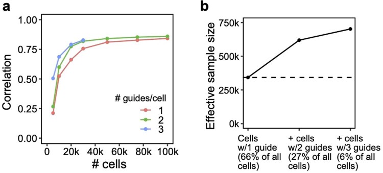
Extended Data Fig. 7 Additional signal in cells containing multiple guides in a conventional 1,130 gene Perturb-seq screen in mouse BMDCs. These cells would normally be discarded before analysis. (a) Correlation of top 10,000 estimated effects with held-out validation (y-axis) when varying cell count (x-axis). (b) Increase in effective sample size in cells (y-axis) when including cells containing 2 or 3 guides (x-axis). Effective sample size for cells with 2 or 3 guides is computed as the number of single-guide containing cells needed to achieve the same held-out validation accuracy (from a).
Extended Data Fig. 7 Additional signal in cells containing multiple guides in a conventional 1,130 gene Perturb-seq screen in mouse BMDCs. These cells would normally be discarded before analysis. (a) Correlation of top 10,000 estimated effects with held-out validation (y-axis) when varying cell count (x-axis). (b) Increase in effective sample size in cells (y-axis) when including cells containing 2 or 3 guides (x-axis). Effective sample size for cells with 2 or 3 guides is computed as the number of single-guide containing cells needed to achieve the same held-out validation accuracy (from a).CC BY · PubMed Central
Extended Data Fig. 8 Experimental validation of six regulators of the inflammatory response. RAB5C, PGM3, XPR1, and KIDINS220 represent novel regulators of the inflammatory response, while MYD88 and STAT1 were included as positive controls. (a) IL6 concentration (as measured by ELISA) in LPS-stimulated THP1 cells infected with single guides. Two guides were included for each target (excluding XPR1, which only has one guide due to all cells receiving the other guide dying). Individual bars represent guides, while individual points represent experimental replicates. (b) Left: Log fold changes of IL6 protein in cells receiving perturbations (averaged across the two guides for each target) relative to non-targeting controls. Right: Mean log fold change of expression of genes in P1 (inflammatory program, see Fig. 5d).
Extended Data Fig. 8 Experimental validation of six regulators of the inflammatory response. RAB5C, PGM3, XPR1, and KIDINS220 represent novel regulators of the inflammatory response, while MYD88 and STAT1 were included as positive controls. (a) IL6 concentration (as measured by ELISA) in LPS-stimulated THP1 cells infected with single guides. Two guides were included for each target (excluding XPR1, which only has one guide due to all cells receiving the other guide dying). Individual bars represent guides, while individual points represent experimental replicates. (b) Left: Log fold changes of IL6 protein in cells receiving perturbations (averaged across the two guides for each target) relative to non-targeting controls. Right: Mean log fold change of expression of genes in P1 (inflammatory program, see Fig. 5d).CC BY · PubMed Central
Extended Data Fig. 9 Additional simulations. (a) Performance of cell/guide pooling when varying sequencing depth (X-axis). Y-axis: correlation of the top 10,000 most significant effects with the true effects. (b) Performance of guide pooling when simulating cells with a fixed number of guides per cell (left; matching the simulation in Extended Data Fig. 6) or when simulating cells with number of guides following a zero-truncated Poisson distribution with mean guides/cell matching the left plot. (c) Performance of guide pooling vs. the efficiency of all guides (x-axis). Guide efficiency is simulated as the proportion of guides that had the intended effect on their target. For example, for a guide efficiency of 0.8, 20% of guides were randomly selected to have no downstream effects. (d) Performance of guide pooling when efficiency within cells decays as a function of the number of guides per cell. Left: 5 different simulated decay scenarios, where the efficiency per cell = e−λ(x−1) and x is the number of guides in the cell. Right: Performance of guide pooling across different # of guides/cell for these 5 scenarios.
Extended Data Fig. 9 Additional simulations. (a) Performance of cell/guide pooling when varying sequencing depth (X-axis). Y-axis: correlation of the top 10,000 most significant effects with the true effects. (b) Performance of guide pooling when simulating cells with a fixed number of guides per cell (left; matching the simulation in Extended Data Fig. 6) or when simulating cells with number of guides following a zero-truncated Poisson distribution with mean guides/cell matching the left plot. (c) Performance of guide pooling vs. the efficiency of all guides (x-axis). Guide efficiency is simulated as the proportion of guides that had the intended effect on their target. For example, for a guide efficiency of 0.8, 20% of guides were randomly selected to have no downstream effects. (d) Performance of guide pooling when efficiency within cells decays as a function of the number of guides per cell. Left: 5 different simulated decay scenarios, where the efficiency per cell = e−λ(x−1) and x is the number of guides in the cell. Right: Performance of guide pooling across different # of guides/cell for these 5 scenarios.CC BY · PubMed Central
Extended Data Fig. 10 Theoretical number of cells needed to learn pairwise interactions at different levels of guide pooling. Number of total perturbations (x-axis) vs. number of cells needed to learn second-order interaction effects between all pairs of perturbation (y-axis), based on the formula N = 400 * C(p, 2) / C(k, 2), where N is the number of cells, p is the number of perturbations, and k the number of guides per cell.
Extended Data Fig. 10 Theoretical number of cells needed to learn pairwise interactions at different levels of guide pooling. Number of total perturbations (x-axis) vs. number of cells needed to learn second-order interaction effects between all pairs of perturbation (y-axis), based on the formula N = 400 * C(p, 2) / C(k, 2), where N is the number of cells, p is the number of perturbations, and k the number of guides per cell.CC BY · PubMed Central

Verification

Claims the paper makes

The claims and statistics of this paper haven’t been checked yet.

Run the check — free, no account needed. It reads the open-access text and checks the sources it cites.

A few free checks a day · papers already verified open instantly · results are public

Claims other papers make about this one

Each is checked against this paper’s own text: does it say what the citing paper says it does?

Self-check

Percentages, sums and reported differences re-computed from the paper’s own numbers.

The self-check needs the paper’s full text.

Citations

Cites

Show all 91 references

Research works printed but not linked: 2

  1. Sharan, V., Tai, K. S., Bailis, P. & Valiant, G. Compressed factorization: fast and accurate low-rank factorization of compressively-sensed data. In Proc. of the 36th International Conference on Machine Learning 5690–5700 (PMLR, 2019).
  2. Mairal, J., Bach, F., Ponce, J. & Sapiro, G. Online learning for matrix factorization and sparse coding. J. Mach. Learn. Res. 11, 19–60 (2010).

Cited by

See all 120

Metadata

Authors
Yao, D., Binan, L., Bezney, J., Simonton, B., Freedman, J., Frangieh, C. J., Dey, K., Geiger-Schuller, K., Eraslan, B., Gusev, A., Regev, A., & Cleary, B.
Affiliations
  • Harvard University (US)
  • Broad Institute (US)
  • Memorial Sloan Kettering Cancer Center (US)
  • Genentech (US)
  • Boston University (US)
Corresponding author
Cleary, Brian
Venue
Nature Biotechnology
Published
2023-10-23
Volume
42
Issue
8
Pages
1282-1295
ISSN
  • 0733-222X (ISSN-L)
  • 1087-0156
  • 1546-1696
OpenAlex
W4387880996
Cited by
101
References
91
Citations by year
2026: 34 · 2025: 43 · 2024: 24
FWCI
9.00
Type
journal article
Language
en
Open access
Licence
Locations
  • Nature Biotechnology (publishedVersion, cc-by)
  • PubMed Central (publishedVersion, cc-by)
  • PubMed (publishedVersion)
  • Digital Access to Scholarship at Harvard (DASH) (Harvard University) (submittedVersion, cc-by)
Funders
  • National Science Foundation (1745303)
  • U.S. Department of Health & Human Services | National Institutes of Health (R00HG012203, P30 CA008748, HG006399)
  • Josie Robertson Investigators Program
  • U.S. Department of Health & Human Services | NIH | National Human Genome Research Institute (RM1HG006193)
  • Broad Fellows program Merkin Institute Fellowship
Topics
  • Life Sciences › Biochemistry, Genetics and Molecular Biology › Molecular Biology › CRISPR and Genetic Engineering
  • Life Sciences › Biochemistry, Genetics and Molecular Biology › Molecular Biology › Single-cell and spatial transcriptomics
  • Life Sciences › Biochemistry, Genetics and Molecular Biology › Molecular Biology › Gene Regulatory Network Analysis
Keywords
Perturb-seq, CRISPR screen, single-cell RNA sequencing, regulatory circuits, genetic interactions, cost reduction, sparse structure, functional genomics
MeSH terms
Algorithms, Genetic Testing, Humans, Sequence Analysis, RNA, Genomics, Gene Regulatory Networks, Genome-Wide Association Study, Single-Cell Analysis, CRISPR-Cas Systems

About these checks

Registry, retraction, Cites and statistics results are computed, not judged, with one exception: a printed reference that no index lists is read once by a model before it counts as a citation error. Claims are extracted by a model and kept only when their quote appears verbatim in the text; each cited source is then checked, with a model’s help, for whether it says what the claim relies on. Those verdicts can be wrong — read the claim’s quote and the cited source before relying on one.

Statistics and arithmetic are recomputed, not judged.

Confidence bands are shown only for fields calibrated on our annotated test set. None is calibrated yet, so no band is shown.

What counts as a claim ›How we measure confidence ›How we check this ›

Are you an author, or do you see a problem with this page? Request a review

How to cite

Cite CoChat for the checks on this page, and the paper for its own findings.

This page
CoChat. (2026). Citation check: Scalable genetic screening for regulatory circuits using compressed Perturb-seq. https://app.cochat.ai/papers/10.1038/s41587-023-01964-9
The paper
Yao, D., Binan, L., Bezney, J., Simonton, B., Freedman, J., Frangieh, C. J., Dey, K., Geiger-Schuller, K., Eraslan, B., Gusev, A., Regev, A., & Cleary, B. (2024). Scalable genetic screening for regulatory circuits using compressed Perturb-seq. Nature Biotechnology. https://doi.org/10.1038/s41587-023-01964-9

Data sources

Bibliographic data: Semantic Scholar, OpenAlex, Crossref.

Contains information from the Semantic Scholar Academic Graph Datasets, made available under the ODC Attribution License (ODC-BY 1.0).

Semantic Scholar’s data is described in: Kinney, R., et al. (2023). The Semantic Scholar Open Data Platform. arXiv:2301.10140.