Student or educator? Sign up with your school email and get 6 months of Pro free.
CoChat

The DOI matches its Crossref record; 68 of the 69 references it cites were found in a registry or an index.

Introducing a Bayesian model of selective attention based on active inference

Open access
Mirza, M. Berk, Adams, Rick A., Friston, Karl, Parr, Thomas · 2019 · Scientific Reports

Abstract

Information gathering comprises actions whose (sensory) consequences resolve uncertainty (i.e., are salient). In other words, actions that solicit salient information cause the greatest shift in beliefs (i.e., information gain) about the causes of our sensations. However, not all information is relevant to the task at hand: this is especially the case in complex, naturalistic scenes. This paper introduces a formal model of selective attention based on active inference and contextual epistemic foraging. We consider a visual search task with a special emphasis on goal-directed and task-relevant exploration. In this scheme, attention modulates the expected fidelity (precision) of the mapping between observations and hidden states in a state-dependent or context-sensitive manner. This ensures task-irrelevant observations have little expected information gain, and so the agent – driven to reduce expected surprise (i.e., uncertainty) – does not actively seek them out. Instead, it selectively samples task-relevant observations, which inform (task-relevant) hidden states. We further show, through simulations, that the atypical exploratory behaviours in conditions such as autism and anxiety may be due to a failure to appropriately modulate sensory precision in a context-specific way.

Overview

The claims and statistics of this paper haven’t been checked yet.

Free: it reads the open-access text and checks the first 5 claims that cite a source we can check. Create a free account to check every claim.

A few free checks a day · papers already verified open instantly · results are public

Integrity signals

Registry

Crossref · 10.1038/s41598-019-50138-8

Cites

68 of 68 references verified0 citation errors · 0 not checkable

Statistics

Figures

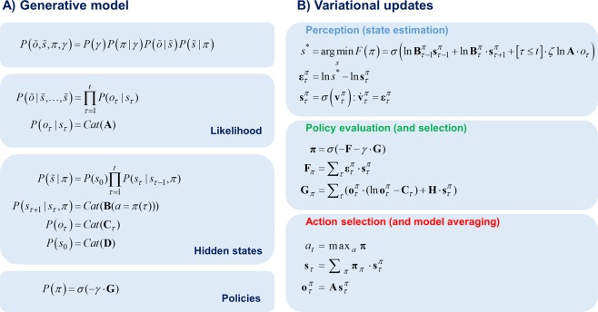
Figure 1 Markovian generative model (A) The joint probability distribution of outcomes and their hidden causes defines the generative model. Here, o˜ corresponds to the sequence of observations o˜=([o1,o2,...,oT])^T over time. Similarly, s˜ represents the sequence of hidden states s˜=([s1,s2,...,sT])^T over time. The generative model comprises a mapping from the hidden states to outcomes (expressed in terms of the likelihood matrix A) and a mapping from the previous hidden state to the next (expressed in terms of the transition matrix B). The notation C at denotes categorical distributions. The transition matrix B is a function of action (a) where action is sampled from the beliefs about the policies (π) for the time step τ. The precision term (γ) mediates the confidence placed in policy selection. The expected free energy (G) expresses how likely a policy is. The prior preference matrix (C) mediates how much one outcome is preferred relative to other outcomes. The initial state probability vector (D) encodes the probability of states at the initial time step P(s0). (B) The belief update equations shown in this panel summarise the variational message passing. Belief updates occur through three phases, namely perception, policy evaluation and action selection. In the perception phase a gradient descent on the state prediction errors ετ^π=−dF/dsτ^π is used to infer the most likely hidden states that generated the observed outcomes. Here s* corresponds to the optimal solution to the state estimation problem, whereas sτ^π corresponds to the current beliefs about states. The updates over the beliefs about states are iterated, using gradient descent, until the state prediction errors are minimised ετ^π≈0. A softmax function is applied to vτ^π=lnsτ^π to obtain a probability distribution over the states. In the first equation, the precision of the likelihood matrix ζ mediates how much the observed outcomes influence the updates over the states (e.g. none when ζ = 0). In the policy evaluation phase, policies π are evaluated in terms of their expected free energy G weighted by its precision γ – and in terms of the free energy based upon previous observations F (please see the text for a more detailed discussion of G and F). Finally, in the action selection phase an action is sampled from the most likely policy π (i.e. policy with the highest posterior probability). The subsequent equation shows that the beliefs about the states sτ are obtained by taking the expectation of beliefs about the states expected under policies sτ^π with respect to the beliefs about the policies π. The final equation shows that the outcomes expected under a policy oτ^π at time step τ are obtained by taking the expectation of the likelihood matrix A with respect to the beliefs about the hidden states under policies sτ^π.
Figure 1 Markovian generative model (A) The joint probability distribution of outcomes and their hidden causes defines the generative model. Here, o˜ corresponds to the sequence of observations o˜=([o1,o2,...,oT])^T over time. Similarly, s˜ represents the sequence of hidden states s˜=([s1,s2,...,sT])^T over time. The generative model comprises a mapping from the hidden states to outcomes (expressed in terms of the likelihood matrix A) and a mapping from the previous hidden state to the next (expressed in terms of the transition matrix B). The notation C at denotes categorical distributions. The transition matrix B is a function of action (a) where action is sampled from the beliefs about the policies (π) for the time step τ. The precision term (γ) mediates the confidence placed in policy selection. The expected free energy (G) expresses how likely a policy is. The prior preference matrix (C) mediates how much one outcome is preferred relative to other outcomes. The initial state probability vector (D) encodes the probability of states at the initial time step P(s0). (B) The belief update equations shown in this panel summarise the variational message passing. Belief updates occur through three phases, namely perception, policy evaluation and action selection. In the perception phase a gradient descent on the state prediction errors ετ^π=−dF/dsτ^π is used to infer the most likely hidden states that generated the observed outcomes. Here s* corresponds to the optimal solution to the state estimation problem, whereas sτ^π corresponds to the current beliefs about states. The updates over the beliefs about states are iterated, using gradient descent, until the state prediction errors are minimised ετ^π≈0. A softmax function is applied to vτ^π=lnsτ^π to obtain a probability distribution over the states. In the first equation, the precision of the likelihood matrix ζ mediates how much the observed outcomes influence the updates over the states (e.g. none when ζ = 0). In the policy evaluation phase, policies π are evaluated in terms of their expected free energy G weighted by its precision γ – and in terms of the free energy based upon previous observations F (please see the text for a more detailed discussion of G and F). Finally, in the action selection phase an action is sampled from the most likely policy π (i.e. policy with the highest posterior probability). The subsequent equation shows that the beliefs about the states sτ are obtained by taking the expectation of beliefs about the states expected under policies sτ^π with respect to the beliefs about the policies π. The final equation shows that the outcomes expected under a policy oτ^π at time step τ are obtained by taking the expectation of the likelihood matrix A with respect to the beliefs about the hidden states under policies sτ^π.CC BY · PubMed Central
Figure 2 Contextual exploration task (A) A scene can be categorised in two ways, either by its colour or its shape. The categories are shown on the left and on top when the rule (context) is to categorise the scene in terms of its colour and shape, respectively. (B) The sequence of observations illustrates exploration of an exemplar scene. In the beginning, each quadrant is greyed out (t = 1). Attending to (i.e. looking at) each quadrant reveals its content. In this case, the order of explored locations is top left (t = 2), bottom left (t = 3) and top right quadrants (t = 4).
Figure 2 Contextual exploration task (A) A scene can be categorised in two ways, either by its colour or its shape. The categories are shown on the left and on top when the rule (context) is to categorise the scene in terms of its colour and shape, respectively. (B) The sequence of observations illustrates exploration of an exemplar scene. In the beginning, each quadrant is greyed out (t = 1). Attending to (i.e. looking at) each quadrant reveals its content. In this case, the order of explored locations is top left (t = 2), bottom left (t = 3) and top right quadrants (t = 4).CC BY · PubMed Central
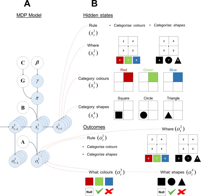
Figure 3 Structure of the generative model – colour/shape task (A) This panel shows the graphical representation of the MDP model and the conditional dependencies among the terms in the model. The structure of the environment is expressed in terms of the transition and likelihood matrices. The likelihood matrix (A) is a mapping from the hidden states (st) to the outcomes (ot). The state transitions are mediated by the transition matrix (B) which expresses how likely the current state (st) is given the previous state (st−1). Crucially, the transition matrix is a function of action which can be sampled from the beliefs about the policies. The beliefs about the policies (π) depend on the expected free energy (G) and the precision of policy selection (γ). The expected free energy comprises extrinsic and epistemic values. Extrinsic value is a function of the prior preference matrix (C) which encodes how much one outcome is expected relative to another. Precision of policy selection (γ) is a function of the temperature term (β). The smaller the temperature the more deterministic the policy selection becomes. (B) This panel shows the four sets of hidden states and outcome modalities in the colour/shape task. There are four sets of hidden states, namely Rule, Where, Category: colours and Category: shapes. There are four outcome modalities, namely Rule, Where, What: colours and What: shapes.
Figure 3 Structure of the generative model – colour/shape task (A) This panel shows the graphical representation of the MDP model and the conditional dependencies among the terms in the model. The structure of the environment is expressed in terms of the transition and likelihood matrices. The likelihood matrix (A) is a mapping from the hidden states (st) to the outcomes (ot). The state transitions are mediated by the transition matrix (B) which expresses how likely the current state (st) is given the previous state (st−1). Crucially, the transition matrix is a function of action which can be sampled from the beliefs about the policies. The beliefs about the policies (π) depend on the expected free energy (G) and the precision of policy selection (γ). The expected free energy comprises extrinsic and epistemic values. Extrinsic value is a function of the prior preference matrix (C) which encodes how much one outcome is expected relative to another. Precision of policy selection (γ) is a function of the temperature term (β). The smaller the temperature the more deterministic the policy selection becomes. (B) This panel shows the four sets of hidden states and outcome modalities in the colour/shape task. There are four sets of hidden states, namely Rule, Where, Category: colours and Category: shapes. There are four outcome modalities, namely Rule, Where, What: colours and What: shapes.CC BY · PubMed Central
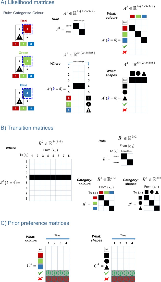
Figure 4 ABC of generative model. This figure shows the likelihood, transition and prior preference matrices used in the colour/shape task. (A) The colour category of the scenes shown on the left is determined purely by the colour in location 4 (top right quadrant). The panels on the right show the likelihood (A) matrices for location k = 4. The likelihood matrices encode the probability of outcomes (ot) given the hidden states (st). The first likelihood matrix A1 (Rule) signals what the rule is, either categorise colour or shape. The second likelihood matrix A2 (Where) signals the sampled location on the scene, one of eight locations. The third likelihood matrix A3 (What: colours) encode the probability of colours red, green and blue under different colour categories red, green and blue. The final likelihood matrix A4 (What: shapes) encode the probability of shapes square, circle and triangle under different shape categories square, circle and triangle. Because the colour and shape are separate modalities, the probability of colour and shape objects are encoded by separate likelihood matrices A3 and A4. The likelihood matrix under the colour modality for location 4 A3(k = 4) shows that the colour category of a scene is purely determined by the colours in this location; however, under the shape modality A4(k = 4) the object in this location does not provide any information about the shape category, i.e. null. (B) This panel shows the transition matrices. All the transition matrices are identity matrices except for the action dependent transition matrix B2, which encodes the most likely location to be sampled as a function of action, e.g. B2(k = 4) shows that under action 4, the top right quadrant is the most likely location to be sampled at the next time step. The identity transition matrices B1 (Rule), B3 (Category: colours) and B4 (Category: shapes) express the fact that the rule and the colour and shape objects do not change in the course of a trial. C) The prior preference matrices are shown in this panel. The prior preference matrices encode how much one outcome is preferred relative to other outcomes as a function of time. The only definitive preferences are defined over the columns of C3 (What: colours) and C4 (What: shapes). Under both C3 and C4 the utility of making a right categorisation and wrong categorisation is +2 and −4 natural units, respectively. With these utilities (i.e. log odds) the agent expects to categorise a scene correctly, while avoiding an incorrect categorisation.
Figure 4 ABC of generative model. This figure shows the likelihood, transition and prior preference matrices used in the colour/shape task. (A) The colour category of the scenes shown on the left is determined purely by the colour in location 4 (top right quadrant). The panels on the right show the likelihood (A) matrices for location k = 4. The likelihood matrices encode the probability of outcomes (ot) given the hidden states (st). The first likelihood matrix A1 (Rule) signals what the rule is, either categorise colour or shape. The second likelihood matrix A2 (Where) signals the sampled location on the scene, one of eight locations. The third likelihood matrix A3 (What: colours) encode the probability of colours red, green and blue under different colour categories red, green and blue. The final likelihood matrix A4 (What: shapes) encode the probability of shapes square, circle and triangle under different shape categories square, circle and triangle. Because the colour and shape are separate modalities, the probability of colour and shape objects are encoded by separate likelihood matrices A3 and A4. The likelihood matrix under the colour modality for location 4 A3(k = 4) shows that the colour category of a scene is purely determined by the colours in this location; however, under the shape modality A4(k = 4) the object in this location does not provide any information about the shape category, i.e. null. (B) This panel shows the transition matrices. All the transition matrices are identity matrices except for the action dependent transition matrix B2, which encodes the most likely location to be sampled as a function of action, e.g. B2(k = 4) shows that under action 4, the top right quadrant is the most likely location to be sampled at the next time step. The identity transition matrices B1 (Rule), B3 (Category: colours) and B4 (Category: shapes) express the fact that the rule and the colour and shape objects do not change in the course of a trial. C) The prior preference matrices are shown in this panel. The prior preference matrices encode how much one outcome is preferred relative to other outcomes as a function of time. The only definitive preferences are defined over the columns of C3 (What: colours) and C4 (What: shapes). Under both C3 and C4 the utility of making a right categorisation and wrong categorisation is +2 and −4 natural units, respectively. With these utilities (i.e. log odds) the agent expects to categorise a scene correctly, while avoiding an incorrect categorisation.CC BY · PubMed Central
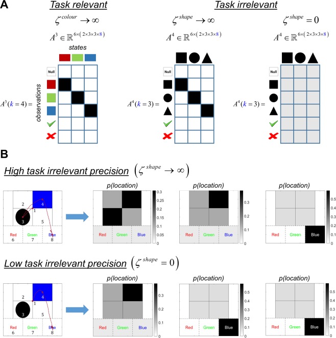
Figure 5 Contextual exploration In this figure, the rule is to categorise a scene in terms of its colour. The objects that resolve uncertainty about the colour category are task-relevant, and the objects that resolve uncertainty about the shape category are task-irrelevant. (A) The likelihood matrix on the left shows the mapping between the task-relevant objects and categories (in this case colour objects and categories), under high precision ζcolour → ∞. The likelihood matrices in the middle and right panels show how the mapping between the task-irrelevant objects and the categories (in this case shape objects and categories) change under two levels of precision ζshape. Under a high precision ζshape → ∞ this mapping is very precise, however under a low precision ζshape = 0 it becomes very ambiguous. When this mapping is imprecise the agent no longer acts to resolve uncertainty about the task-irrelevant category. The task-relevant and irrelevant likelihood matrices are illustrated for locations 3 and 4, because these are the only locations that hold the objects that resolve uncertainty about the shape and colour categories, respectively. The precision term ζcolour is used to change the mapping between colour objects and categories in the same way when the rule is categorise shape. (B) The upper and lower left panels show how the exploratory behaviour changes under two levels of task-irrelevant precisions ζshape → ∞ and ζshape = 0, while keeping task-relevant precision high ζcolour → ∞. The subsequent panels show how likely an agent is to sample a location during the course of a trial, expressed in terms of prior probabilities for each policy. At the beginning of each trial, the agent fixates at the centre of the screen (location 1). Under high task-irrelevant ζshape → ∞ and task-relevant ζcolour → ∞ precisions, the agent finds that it is equally likely to attend to the task-relevant colour objects in location 4 as the task-irrelevant shape objects in location 3, in the beginning. The agent first attends to location 3 where it finds a circle and then attends to location 4, where it finds the colour blue. Subsequently the scene is categorised as blue. Under a low task-irrelevant precision ζshape = 0 and high task-relevant precision ζcolour → ∞ the agent infers that the only location that matters is location 4, which holds the task-relevant colour objects. In the next time step it attends to location 4 and finds the colour blue and subsequently categorises the scene as blue.
Figure 5 Contextual exploration In this figure, the rule is to categorise a scene in terms of its colour. The objects that resolve uncertainty about the colour category are task-relevant, and the objects that resolve uncertainty about the shape category are task-irrelevant. (A) The likelihood matrix on the left shows the mapping between the task-relevant objects and categories (in this case colour objects and categories), under high precision ζcolour → ∞. The likelihood matrices in the middle and right panels show how the mapping between the task-irrelevant objects and the categories (in this case shape objects and categories) change under two levels of precision ζshape. Under a high precision ζshape → ∞ this mapping is very precise, however under a low precision ζshape = 0 it becomes very ambiguous. When this mapping is imprecise the agent no longer acts to resolve uncertainty about the task-irrelevant category. The task-relevant and irrelevant likelihood matrices are illustrated for locations 3 and 4, because these are the only locations that hold the objects that resolve uncertainty about the shape and colour categories, respectively. The precision term ζcolour is used to change the mapping between colour objects and categories in the same way when the rule is categorise shape. (B) The upper and lower left panels show how the exploratory behaviour changes under two levels of task-irrelevant precisions ζshape → ∞ and ζshape = 0, while keeping task-relevant precision high ζcolour → ∞. The subsequent panels show how likely an agent is to sample a location during the course of a trial, expressed in terms of prior probabilities for each policy. At the beginning of each trial, the agent fixates at the centre of the screen (location 1). Under high task-irrelevant ζshape → ∞ and task-relevant ζcolour → ∞ precisions, the agent finds that it is equally likely to attend to the task-relevant colour objects in location 4 as the task-irrelevant shape objects in location 3, in the beginning. The agent first attends to location 3 where it finds a circle and then attends to location 4, where it finds the colour blue. Subsequently the scene is categorised as blue. Under a low task-irrelevant precision ζshape = 0 and high task-relevant precision ζcolour → ∞ the agent infers that the only location that matters is location 4, which holds the task-relevant colour objects. In the next time step it attends to location 4 and finds the colour blue and subsequently categorises the scene as blue.CC BY · PubMed Central
Figure 6 Learning the locations of the features in Yarbus’ task. (A) The painting An Unexpected Visitor by Ilya Repin is shown on the left. The right panel highlights 13 locations that can furnish information about either material circumstances of the family or the ages of the people in the painting. The first location is the centre of the scene. Furniture and clothing appear at locations 2, 4, 6, 9, 10 and 11. Faces appear at locations 3, 5, 7, 8, 12 and 13. For illustrative purposes, location 3 has been chosen to show that one can see young, middle aged or old faces in locations a face can appear. Location 6 has been chosen to show that one can see an antique, a modest or a common chair in locations a piece of furniture (or man’s/woman’s clothing) can appear. (B) This panel shows a scene in which locations 2 and 4 hold a modest and a common chair, respectively, whereas locations 6, 9, 10 and 11 locate antique chairs. Similarly, locations 3 and 5 hold a middle aged and an old face, respectively, whereas locations 7, 8, 12 and 13 locate young faces. (C) Agents learn the locations of the features shown in panel B by accumulating counts for each state-outcome pair, where the novelty term (see Eq. 4.) drives behaviour such that exposure to these novel combinations is assured. This enables the agent to learn the (likelihood) mapping from locations to objects A3 and faces A4 in the course of free visual exploration. The likelihood matrices – on the top – show that the agent initially has no knowledge of which features are located where. The matrices in the middle show that the agent starts to learn the locations of the objects and faces after an initial scan of the scene. The matrices at the bottom show that after a thorough exploration of the scene, the agent has precise knowledge of the object locations. The painting Unexpected Visitors by Ilya Repin has been downloaded from https://commons.wikimedia.org/w/index.php?title=File:Ilya_Repin_Unexpected_visitors.jpg 71. The cartoon faces and the pictures of the chairs in this figure have been downloaded from https://pixabay.com/.
Figure 6 Learning the locations of the features in Yarbus’ task. (A) The painting An Unexpected Visitor by Ilya Repin is shown on the left. The right panel highlights 13 locations that can furnish information about either material circumstances of the family or the ages of the people in the painting. The first location is the centre of the scene. Furniture and clothing appear at locations 2, 4, 6, 9, 10 and 11. Faces appear at locations 3, 5, 7, 8, 12 and 13. For illustrative purposes, location 3 has been chosen to show that one can see young, middle aged or old faces in locations a face can appear. Location 6 has been chosen to show that one can see an antique, a modest or a common chair in locations a piece of furniture (or man’s/woman’s clothing) can appear. (B) This panel shows a scene in which locations 2 and 4 hold a modest and a common chair, respectively, whereas locations 6, 9, 10 and 11 locate antique chairs. Similarly, locations 3 and 5 hold a middle aged and an old face, respectively, whereas locations 7, 8, 12 and 13 locate young faces. (C) Agents learn the locations of the features shown in panel B by accumulating counts for each state-outcome pair, where the novelty term (see Eq. 4.) drives behaviour such that exposure to these novel combinations is assured. This enables the agent to learn the (likelihood) mapping from locations to objects A3 and faces A4 in the course of free visual exploration. The likelihood matrices – on the top – show that the agent initially has no knowledge of which features are located where. The matrices in the middle show that the agent starts to learn the locations of the objects and faces after an initial scan of the scene. The matrices at the bottom show that after a thorough exploration of the scene, the agent has precise knowledge of the object locations. The painting Unexpected Visitors by Ilya Repin has been downloaded from https://commons.wikimedia.org/w/index.php?title=File:Ilya_Repin_Unexpected_visitors.jpg 71. The cartoon faces and the pictures of the chairs in this figure have been downloaded from https://pixabay.com/.CC BY · PubMed Central
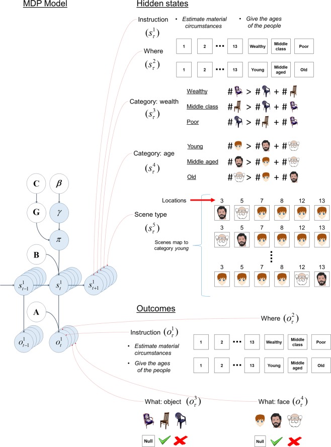
Figure 7 Structure of the generative model – Yarbus’ task. The structure of the generative model is shown on the left – see Fig. 3A for a detailed description. On the right are the five sets of hidden states and four outcome modalities in our MDP version of Yarbus’ task. There are five sets of hidden states, namely Instruction, Where, Category: wealth, Category: age and Scene type. There are four outcome modalities, namely Instruction, Where, What: object and What: face. See the main text for details. The cartoon faces and the pictures of the chairs in this figure have been downloaded from https://pixabay.com/.
Figure 7 Structure of the generative model – Yarbus’ task. The structure of the generative model is shown on the left – see Fig. 3A for a detailed description. On the right are the five sets of hidden states and four outcome modalities in our MDP version of Yarbus’ task. There are five sets of hidden states, namely Instruction, Where, Category: wealth, Category: age and Scene type. There are four outcome modalities, namely Instruction, Where, What: object and What: face. See the main text for details. The cartoon faces and the pictures of the chairs in this figure have been downloaded from https://pixabay.com/.CC BY · PubMed Central
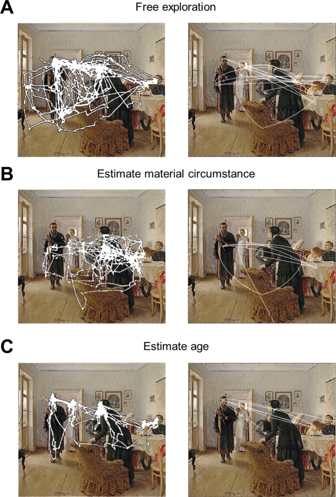
Figure 8 Yarbus’ free exploration task and simulations (A) The panel on the left shows how real subjects explored the painting freely in Yarbus’ experiment, whereas the right panel shows the simulated exploratory behaviour of a context naïve agent (unaware of the instructions and thus exploring the scene freely). The agent starts exploring from the centre of the scene (location 1) (B) The panels on the left and right show how the real subjects and the agent explore the painting under the instructions estimate material circumstances of the family. (C) The panels on the left and right show responses when exploring the painting under the instructions give the ages of the people. The painting Unexpected Visitors by Ilya Repin has been downloaded from https://commons.wikimedia.org/w/index.php?title=File:Ilya_Repin_Unexpected_visitors.jpg 71. The panels on the left show the scanpaths of the subjects that explored this painting in Yarbus’ work (see Yarbus’ work6 for the originals of the scanpaths). The scan-paths available on the below link are superimposed on the painting itself to produce the panels on the right: https://commons.wikimedia.org/w/index.php?title=File:Yarbus_The_Visitor.jpg 72.
Figure 8 Yarbus’ free exploration task and simulations (A) The panel on the left shows how real subjects explored the painting freely in Yarbus’ experiment, whereas the right panel shows the simulated exploratory behaviour of a context naïve agent (unaware of the instructions and thus exploring the scene freely). The agent starts exploring from the centre of the scene (location 1) (B) The panels on the left and right show how the real subjects and the agent explore the painting under the instructions estimate material circumstances of the family. (C) The panels on the left and right show responses when exploring the painting under the instructions give the ages of the people. The painting Unexpected Visitors by Ilya Repin has been downloaded from https://commons.wikimedia.org/w/index.php?title=File:Ilya_Repin_Unexpected_visitors.jpg 71. The panels on the left show the scanpaths of the subjects that explored this painting in Yarbus’ work (see Yarbus’ work6 for the originals of the scanpaths). The scan-paths available on the below link are superimposed on the painting itself to produce the panels on the right: https://commons.wikimedia.org/w/index.php?title=File:Yarbus_The_Visitor.jpg 72.CC BY · PubMed Central
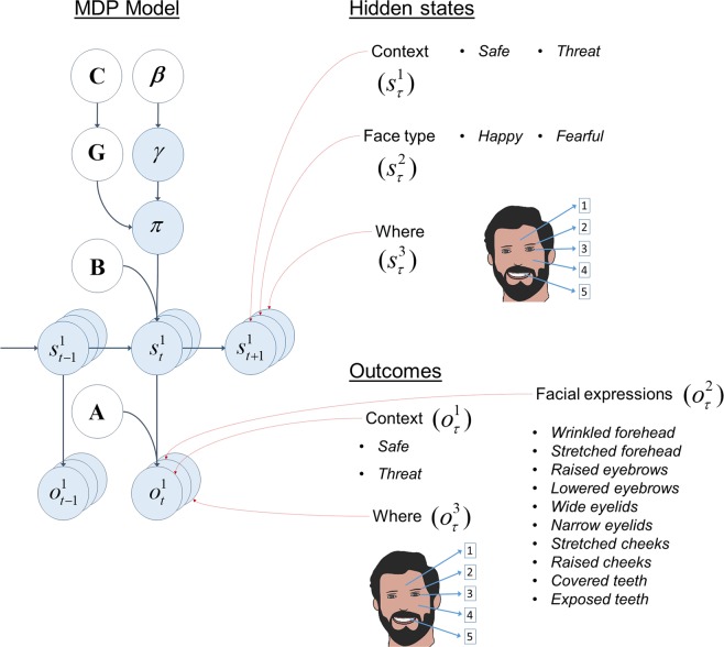
Figure 9 Structure of the generative model – Facial expression identification task. The structure of the generative model is shown on the left – see Fig. 3A for a detailed description. The right panel shows that there are three hidden states, namely Context, Face type and Where. There are three outcome modalities, namely Context, Facial expressions and Where. See the main text for details.
Figure 9 Structure of the generative model – Facial expression identification task. The structure of the generative model is shown on the left – see Fig. 3A for a detailed description. The right panel shows that there are three hidden states, namely Context, Face type and Where. There are three outcome modalities, namely Context, Facial expressions and Where. See the main text for details.CC BY · PubMed Central
Figure 10 Empirical results and simulations (A) The left panels report the proportion of fixations on objects and heads when Yarbus’ visual search task is performed by typically developing (TD) adults and people with a diagnosis of autism spectrum disorder (ASD) under the instructions estimate the material circumstances of the family (Task A) and estimate how long the unexpected visitor has been away (Task B). The panels on the right show the simulated proportion of fixations using the MDP model. (B) Healthy people performed a face identification task under different conditions, namely threat of shock (threat) and free from threat of shock (safe). In this task, either a happy or a fearful face is shown on a computer screen. The participants are asked to identify the face as either happy or fearful as quickly as they can. The left panel shows the empirical reaction times (i.e., time it took to identify the facial emotion), whereas the right panel shows the simulated decision times using the MDP model (i.e., the number of facial features the agent attended before identifying the face). See the main text for details. See Benson et al.35 and Robinson et al.37 for the originals of the figures on the left panels of A and B in this figure, respectively. These figures were reproduced with permission from Elsevier and the rights to use these materials have been obtained through Copyright Clearance Centre.
Figure 10 Empirical results and simulations (A) The left panels report the proportion of fixations on objects and heads when Yarbus’ visual search task is performed by typically developing (TD) adults and people with a diagnosis of autism spectrum disorder (ASD) under the instructions estimate the material circumstances of the family (Task A) and estimate how long the unexpected visitor has been away (Task B). The panels on the right show the simulated proportion of fixations using the MDP model. (B) Healthy people performed a face identification task under different conditions, namely threat of shock (threat) and free from threat of shock (safe). In this task, either a happy or a fearful face is shown on a computer screen. The participants are asked to identify the face as either happy or fearful as quickly as they can. The left panel shows the empirical reaction times (i.e., time it took to identify the facial emotion), whereas the right panel shows the simulated decision times using the MDP model (i.e., the number of facial features the agent attended before identifying the face). See the main text for details. See Benson et al.35 and Robinson et al.37 for the originals of the figures on the left panels of A and B in this figure, respectively. These figures were reproduced with permission from Elsevier and the rights to use these materials have been obtained through Copyright Clearance Centre.CC BY · PubMed Central

Verification

Claims the paper makes

The claims and statistics of this paper haven’t been checked yet.

Free: it reads the open-access text and checks the first 5 claims that cite a source we can check. Create a free account to check every claim.

A few free checks a day · papers already verified open instantly · results are public

Claims other papers make about this one

Each is checked against this paper’s own text: does it say what the citing paper says it does?

Self-check

Percentages, sums and reported differences re-computed from the paper’s own numbers.

The self-check needs the paper’s full text.

Citations

Cites

Show all 69 references

Research works printed but not linked: 4

  1. Achanta, R., Hemami, S., Estrada, F. & Susstrunk, S. In Computer vision and pattern recognition, 2009. cvpr 2009. ieee conference on. 1597–1604 (IEEE).
  2. Ma, Y.-F. & Zhang, H.-J. In Proceedings of the eleventh ACM international conference on Multimedia. 374–381 (ACM).
  3. Navalpakkam, V. & Itti, L. In Computer Vision and Pattern Recognition, 2006 IEEE Computer Society Conference on. 2049–2056 (IEEE).
  4. Gao, D. & Vasconcelos, N. In Advances in neural information processing systems. 481–488 (2005).

Cited by

See all 103

Metadata

Authors
Mirza, M. B., Adams, R. A., Friston, K., & Parr, T.
Affiliations
  • Wellcome Centre for Human Neuroimaging (GB)
  • University College London (GB)
Corresponding author
Mirza, M. Berk
Venue
Scientific Reports
Published
2019-09-26
Volume
9
Issue
1
Pages
13915-13915
ISSN
2045-2322 (ISSN-L)
OpenAlex
W2976482801
Cited by
83
References
69
Citations by year
2026: 10 · 2025: 10 · 2024: 14 · 2023: 14 · 2022: 12 · 2021: 12 · 2020: 11
FWCI
5.09
Type
journal article
Language
en
Open access
Licence
Locations
  • Scientific Reports (publishedVersion, cc-by)
  • Europe PMC (PubMed Central) (publishedVersion, cc-by)
  • PubMed Central (publishedVersion, cc-by)
  • PubMed (publishedVersion)
  • DOAJ (DOAJ: Directory of Open Access Journals) (submittedVersion)
  • UCL Discovery (University College London) (submittedVersion)
  • MPG.PuRe (Max Planck Society) (submittedVersion)
Funders
  • Wellcome Trust (088130, 088130/Z/09/Z)
  • National Institute for Health and Care Research (CL-2013-18-003)
  • Academy of Medical Sciences (SGCL13, AMS-SGCL13, AMS‐SGCL13‐Adams)
  • European Commission (642961, HORIZON2020)
  • Rosetrees Trust (173346)
  • University College London Hospitals NHS Foundation Trust
  • Medical Research Council (MR/S007806/1)
  • Research Executive Agency
Topics
  • Life Sciences › Neuroscience › Cognitive Neuroscience › Embodied and Extended Cognition
  • Physical Sciences › Computer Science › Computer Vision and Pattern Recognition › Visual Attention and Saliency Detection
  • Life Sciences › Neuroscience › Cognitive Neuroscience › Visual perception and processing mechanisms
Keywords
selective attention, active inference, visual search, information gain, goal-directed exploration, autism spectrum disorder, anxiety, Bayesian model

About these checks

Registry, retraction, Cites and statistics results are computed, not judged, with one exception: a printed reference that no index lists is read once by a model before it counts as a citation error. Claims are extracted by a model and kept only when their quote appears verbatim in the text; each cited source is then checked, with a model’s help, for whether it says what the claim relies on. Those verdicts can be wrong — read the claim’s quote and the cited source before relying on one.

Statistics and arithmetic are recomputed, not judged.

Confidence bands are shown only for fields calibrated on our annotated test set. None is calibrated yet, so no band is shown.

What counts as a claim ›How we measure confidence ›How we check this ›

Are you an author, or do you see a problem with this page? Request a review

How to cite

Cite CoChat for the checks on this page, and the paper for its own findings.

This page
CoChat. (2026). Citation check: Introducing a Bayesian model of selective attention based on active inference. https://app.cochat.ai/papers/10.1038/s41598-019-50138-8
The paper
Mirza, M. B., Adams, R. A., Friston, K., & Parr, T. (2019). Introducing a Bayesian model of selective attention based on active inference. Scientific Reports. https://doi.org/10.1038/s41598-019-50138-8

Data sources

Bibliographic data: Semantic Scholar, OpenAlex, Crossref.

Contains information from the Semantic Scholar Academic Graph Datasets, made available under the ODC Attribution License (ODC-BY 1.0).

Semantic Scholar’s data is described in: Kinney, R., et al. (2023). The Semantic Scholar Open Data Platform. arXiv:2301.10140.