CoChat

Quantum gravity from causal dynamical triangulations: a review

Open access
Loll, R · 2020 · Classical and Quantum Gravity

The DOI matches its Crossref record; 106 of the 106 references it cites were found in a registry or an index.

Abstract

This topical review gives a comprehensive overview and assessment of recent results in causal dynamical triangulations, a modern formulation of lattice gravity, whose aim is to obtain a theory of quantum gravity nonperturbatively from a scaling limit of the lattice-regularized theory. In this manifestly diffeomorphism-invariant approach one has direct, computational access to a Planckian spacetime regime, which is explored with the help of invariant quantum observables. During the last few years, there have been numerous new and important developments and insights concerning the theory’s phase structure, the roles of time, causality, diffeomorphisms and global topology, the application of renormalization group methods and new observables. We will focus on these new results, primarily in four spacetime dimensions, and discuss some of their geometric and physical implications.

Overview

The claims and statistics of this paper haven’t been checked yet.

Free: it reads the open-access text and checks the first 5 claims that cite a source we can check. Create a free account to check every claim.

A few free checks a day · papers already verified open instantly · results are public

Integrity signals

Registry

Crossref · 10.1088/1361-6382/ab57c7

Cites

106 of 106 references verified0 citation errors · 0 not checkable

Statistics

Figures

Figure 1 Regularized spacetimes in CDT quantum gravity are built from two elementary four-simplices, the (4,1)-simplex (left) and the (3,2)-simplex (right). They differ in their assignments of space- and time-like edges, drawn in blue and red respectively, see [17] for details.
Figure 1 Regularized spacetimes in CDT quantum gravity are built from two elementary four-simplices, the (4,1)-simplex (left) and the (3,2)-simplex (right). They differ in their assignments of space- and time-like edges, drawn in blue and red respectively, see [17] for details.CC-BY · From the PDF
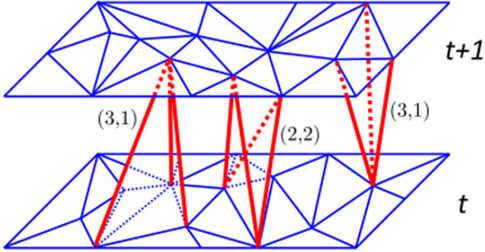
Figure 2 A ' sandwich geometry ' of topology I × ( 2 ) Σ for CDT in 2 + 1 spacetime dimensions. The sandwich consists of a layer of three-simplices (tetrahedra) interpolating between two adjacent spatial slices at times t and t + 1 made up of two-dimensional triangles. The space between the lower and upper triangulation is completely filled with tetrahedra, but for simplicity only three are shown here. (Space-like edges depicted in blue, time-like ones in red.)
Figure 2 A ' sandwich geometry ' of topology I × ( 2 ) Σ for CDT in 2 + 1 spacetime dimensions. The sandwich consists of a layer of three-simplices (tetrahedra) interpolating between two adjacent spatial slices at times t and t + 1 made up of two-dimensional triangles. The space between the lower and upper triangulation is completely filled with tetrahedra, but for simplicity only three are shown here. (Space-like edges depicted in blue, time-like ones in red.)CC-BY · From the PDF
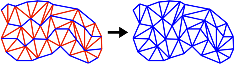
Figure 3 The layered structure of a two-dimensional CDT configuration, with space-like edges drawn in blue and time-like ones in red. Left: CDT geometry consisting of a stack of three sandwiches. The spatial geometries at discrete times t are open chains consisting of a variable number l t > 0 of space-like edges. Right: the corresponding Euclidean geometry after Wick rotation. The underlying lattice structure is unchanged, but all time-like edges have been replaced by space-like ones.
Figure 3 The layered structure of a two-dimensional CDT configuration, with space-like edges drawn in blue and time-like ones in red. Left: CDT geometry consisting of a stack of three sandwiches. The spatial geometries at discrete times t are open chains consisting of a variable number l t > 0 of space-like edges. Right: the corresponding Euclidean geometry after Wick rotation. The underlying lattice structure is unchanged, but all time-like edges have been replaced by space-like ones.CC-BY · From the PDF
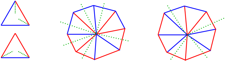
Figure 4 Left: the two elementary Minkowskian building blocks of CDT without preferred foliation in two dimensions; in standard CDT only the lower one is present. Dotted lines indicate light rays through the corner points. Centre: gluing these triangles together can result in local causality violations, like too many light cones meeting at a vertex, as shown. Right: at a causally well-behaved vertex, one crosses exactly four light-like directions when going around the vertex.
Figure 4 Left: the two elementary Minkowskian building blocks of CDT without preferred foliation in two dimensions; in standard CDT only the lower one is present. Dotted lines indicate light rays through the corner points. Centre: gluing these triangles together can result in local causality violations, like too many light cones meeting at a vertex, as shown. Right: at a causally well-behaved vertex, one crosses exactly four light-like directions when going around the vertex.CC-BY · From the PDF
Figure 5 CDT phase diagram spanned by the bare couplings κ 0 and ∆ , consisting of the de Sitter phase C dS , the bifurcation phase Cb , and two unphysical phases A and B . (Fat dots and squares refer to actual measurements.)
Figure 5 CDT phase diagram spanned by the bare couplings κ 0 and ∆ , consisting of the de Sitter phase C dS , the bifurcation phase Cb , and two unphysical phases A and B . (Fat dots and squares refer to actual measurements.)CC-BY · From the PDF
Image 6
CC-BY · From the PDF
Image 7
CC-BY · From the PDF
Figure 8 Measured matrix elements 〈 n | M | s -n 〉 for s = 30 k, at fixed κ 0 = 2.2 and for five different ∆ -values. Since s = m + n stays constant, these measurements illustrate the behaviour of the kinetic part of (18): the smaller ∆ , the more pronounced is the ' bifurcation ' into two Gaussians. The Cb -C dS phase transition (merger to a single Gaussian) appears to lie in the interval ∆ ∈ [ 0.25, 0.3 ] . (Figure reproduced from [76]. CC BY 4.0.)
Figure 8 Measured matrix elements 〈 n | M | s -n 〉 for s = 30 k, at fixed κ 0 = 2.2 and for five different ∆ -values. Since s = m + n stays constant, these measurements illustrate the behaviour of the kinetic part of (18): the smaller ∆ , the more pronounced is the ' bifurcation ' into two Gaussians. The Cb -C dS phase transition (merger to a single Gaussian) appears to lie in the interval ∆ ∈ [ 0.25, 0.3 ] . (Figure reproduced from [76]. CC BY 4.0.)CC-BY · From the PDF
Figure 9 In the bifurcation phase Cb ( ∆ = 0.2 ), the maximal coordination number O max ( t ) : = max [ O ( v ( t ))] jumps to a very large value on every second spatial slice, compared with the situation in the de Sitter phase C dS ( ∆ = 0.5 ). Measurements taken for t tot = 80 , N 41 = 160 k, κ 0 = 2.2 , and averaged over many configurations. (Figure reprinted figure with permission from [87], copyright 2017 by the American Physical Society.)
Figure 9 In the bifurcation phase Cb ( ∆ = 0.2 ), the maximal coordination number O max ( t ) : = max [ O ( v ( t ))] jumps to a very large value on every second spatial slice, compared with the situation in the de Sitter phase C dS ( ∆ = 0.5 ). Measurements taken for t tot = 80 , N 41 = 160 k, κ 0 = 2.2 , and averaged over many configurations. (Figure reprinted figure with permission from [87], copyright 2017 by the American Physical Society.)CC-BY · From the PDF
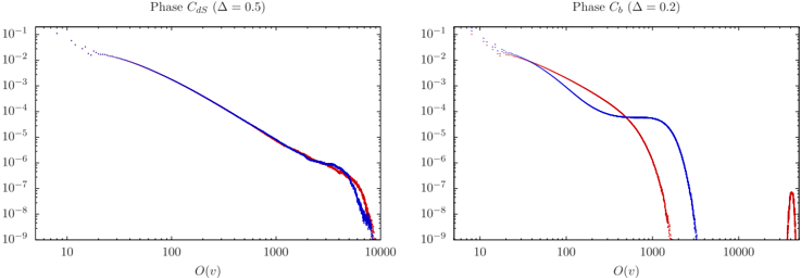
Figure 10 Histograms of the coordination number O ( v ) in the spatial slice containing the vertex with maximal coordination number (red curves) and in a neighbouring spatial slice (blue curves). In the de Sitter phase ( ∆ = 0.5 , left) there is hardly any difference. In the bifurcation phase ( ∆ = 0.2 , right), the singular vertices form a peak in O ( v ) isolated from the rest of the distribution, which is not present in slices without singular vertices. Measurements taken for t tot = 80 , N 41 = 160 k and κ 0 = 2.2 . (Figures courtesy of G ö rlich.)
Figure 10 Histograms of the coordination number O ( v ) in the spatial slice containing the vertex with maximal coordination number (red curves) and in a neighbouring spatial slice (blue curves). In the de Sitter phase ( ∆ = 0.5 , left) there is hardly any difference. In the bifurcation phase ( ∆ = 0.2 , right), the singular vertices form a peak in O ( v ) isolated from the rest of the distribution, which is not present in slices without singular vertices. Measurements taken for t tot = 80 , N 41 = 160 k and κ 0 = 2.2 . (Figures courtesy of G ö rlich.)CC-BY · From the PDF
Figure 11 Schematic illustration of the spacetime geometry inside the bifurcation phase, where the singular vertices present on every second spatial slice align themselves into a chain of diamond-like regions, as shown in the figure on the left. (Figures reproduced from [76]. CC BY 4.0.)
Figure 11 Schematic illustration of the spacetime geometry inside the bifurcation phase, where the singular vertices present on every second spatial slice align themselves into a chain of diamond-like regions, as shown in the figure on the left. (Figures reproduced from [76]. CC BY 4.0.)CC-BY · From the PDF
Image 12
CC-BY · From the PDF
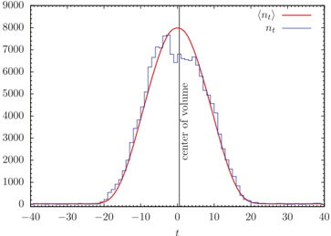
Figure 12 Snapshot of a typical volume configuration nt (blue) and the expectation value 〈 nt 〉 (red), both for spherical slices (left) and toroidal ones (right). All measurements taken at ( κ 0, ∆) = ( 2.2, 0.6 ) , and for N 41 = 160 k and t tot = 80 . (Figures reproduced from [90]. CC BY 4.0.)
Figure 12 Snapshot of a typical volume configuration nt (blue) and the expectation value 〈 nt 〉 (red), both for spherical slices (left) and toroidal ones (right). All measurements taken at ( κ 0, ∆) = ( 2.2, 0.6 ) , and for N 41 = 160 k and t tot = 80 . (Figures reproduced from [90]. CC BY 4.0.)CC-BY · From the PDF
Figure 13 V olume profile 〈 nt 〉 of CDT configurations with t tot = 40 toroidal slices, with fixed spatial volumes ¯ n 1 = 1000 and ¯ n 21 = 7000 . The shaded region indicates the size of the quantum fluctuations of nt around the mean. Measurements taken at ( κ 0, ∆) = ( 2.2, 0.6 ) and κ 4 = 0.9225 . (Figure reproduced from [90]. CC BY 4.0.)
Figure 13 V olume profile 〈 nt 〉 of CDT configurations with t tot = 40 toroidal slices, with fixed spatial volumes ¯ n 1 = 1000 and ¯ n 21 = 7000 . The shaded region indicates the size of the quantum fluctuations of nt around the mean. Measurements taken at ( κ 0, ∆) = ( 2.2, 0.6 ) and κ 4 = 0.9225 . (Figure reproduced from [90]. CC BY 4.0.)CC-BY · From the PDF
Figure 14 Sample volume profiles nt of CDT configurations with t tot = 40 toroidal slices and for N 41 = 40 k display characteristics familiar from phases A and B of the spherical system. (Figures reproduced from [91]. CC BY 4.0.)
Figure 14 Sample volume profiles nt of CDT configurations with t tot = 40 toroidal slices and for N 41 = 40 k display characteristics familiar from phases A and B of the spherical system. (Figures reproduced from [91]. CC BY 4.0.)CC-BY · From the PDF
Figure 15 The phase diagram of CDT quantum gravity with t tot = 4 toroidal slices, from measurements at volume N 41 = 160 k. Phase transitions are marked by solid lines, with shaded areas of the same colour indicating error bars. Dots mark measurement points, with different colours associated to the four different phases. The phase denoted C is the analogue of the de Sitter phase for spherical slices. Dashed black lines indicate extrapolations. (Figure reproduced from [91]. CC BY 4.0.)
Figure 15 The phase diagram of CDT quantum gravity with t tot = 4 toroidal slices, from measurements at volume N 41 = 160 k. Phase transitions are marked by solid lines, with shaded areas of the same colour indicating error bars. Dots mark measurement points, with different colours associated to the four different phases. The phase denoted C is the analogue of the de Sitter phase for spherical slices. Dashed black lines indicate extrapolations. (Figure reproduced from [91]. CC BY 4.0.)CC-BY · From the PDF
Image 17
CC-BY · From the PDF
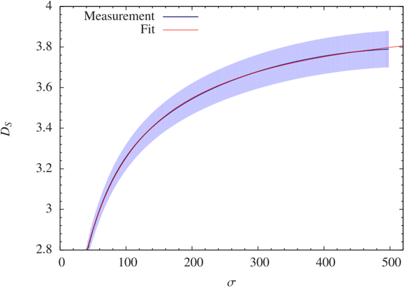
Figure 17 The spectral dimension DS of spacetime as a function of the diffusion time σ , measured at ( κ 0, ∆) = ( 2.2, 0.6 ) , for t tot = 80 and a spacetime volume N 4 = 181 k. The averaged measurements lie along the central curve, together with a superimposed best fit DS ( σ ) = 4.02 -119 / ( 54 + σ ) . The two outer curves represent error bars.
Figure 17 The spectral dimension DS of spacetime as a function of the diffusion time σ , measured at ( κ 0, ∆) = ( 2.2, 0.6 ) , for t tot = 80 and a spacetime volume N 4 = 181 k. The averaged measurements lie along the central curve, together with a superimposed best fit DS ( σ ) = 4.02 -119 / ( 54 + σ ) . The two outer curves represent error bars.CC-BY · From the PDF
Figure 18 The spectral dimension DS of spacetime in phase A , measured at ( κ 0, ∆) = ( 8.0, 0.6 ) , for t tot = 80 and N 41 = 160 k, exhibits a fractal, scale-independent behaviour. (Figure reproduced from [97]. CC BY 4.0.)
Figure 18 The spectral dimension DS of spacetime in phase A , measured at ( κ 0, ∆) = ( 8.0, 0.6 ) , for t tot = 80 and N 41 = 160 k, exhibits a fractal, scale-independent behaviour. (Figure reproduced from [97]. CC BY 4.0.)CC-BY · From the PDF
Figure 19 Effective spectral dimension D eff of spatial slices at ( κ 0, ∆) = ( 5.0, 0.6 ) in phase A , ( 2.2, -0.2 ) in phase B and ( 2.2, 0.6 ) in phase C dS , measured for t tot = 80 , spacetime volume N 41 = 80 k (phases A and C dS ) and N 41 = 16 k (phase B ), and in small bins of n / VS [50]. In the kinematical limit n / VS → 1 the effective dimensions are close to 3, primarily determined by the discrete lattice set-up. (Figure reproduced from [50]. CC BY 4.0.)
Figure 19 Effective spectral dimension D eff of spatial slices at ( κ 0, ∆) = ( 5.0, 0.6 ) in phase A , ( 2.2, -0.2 ) in phase B and ( 2.2, 0.6 ) in phase C dS , measured for t tot = 80 , spacetime volume N 41 = 80 k (phases A and C dS ) and N 41 = 16 k (phase B ), and in small bins of n / VS [50]. In the kinematical limit n / VS → 1 the effective dimensions are close to 3, primarily determined by the discrete lattice set-up. (Figure reproduced from [50]. CC BY 4.0.)CC-BY · From the PDF
Figure 20 Histogram of the invariant angles ( θ 1, θ 2 ) , extracted from Monte Carlo measurements of Wilson loops in CDT [43], matching the functional form (37) up to an overall normalization.
Figure 20 Histogram of the invariant angles ( θ 1, θ 2 ) , extracted from Monte Carlo measurements of Wilson loops in CDT [43], matching the functional form (37) up to an overall normalization.CC-BY · From the PDF
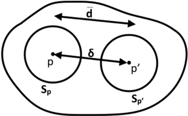
Figure 21 To obtain the local Ricci curvature Ric ( v , v ) associated with a vector v on a smooth Riemannian space, one compares the distance ¯ d of two small nearby spheres Sp and Sp ′ with the distance δ = | v | of their centres p and p ′ , measured along the unique geodesic from p to p ′ in the direction of v .
Figure 21 To obtain the local Ricci curvature Ric ( v , v ) associated with a vector v on a smooth Riemannian space, one compares the distance ¯ d of two small nearby spheres Sp and Sp ′ with the distance δ = | v | of their centres p and p ′ , measured along the unique geodesic from p to p ′ in the direction of v .CC-BY · From the PDF
Figure 22 The normalized average sphere distance ¯ d /δ as a function of δ ∈ [ 0, 2 π ] for three constantly curved model spaces in two dimensions. The analogous curves in higher dimensions look qualitatively similar. The curvature radius has been set to 1 wherever applicable.
Figure 22 The normalized average sphere distance ¯ d /δ as a function of δ ∈ [ 0, 2 π ] for three constantly curved model spaces in two dimensions. The analogous curves in higher dimensions look qualitatively similar. The curvature radius has been set to 1 wherever applicable.CC-BY · From the PDF
Figure 23 Relations in theory space: different ways to derive cosmology from nonperturbative quantum gravity and general relativity.
Figure 23 Relations in theory space: different ways to derive cosmology from nonperturbative quantum gravity and general relativity.CC-BY · From the PDF

Verification

Claims the paper makes

The claims and statistics of this paper haven’t been checked yet.

Free: it reads the open-access text and checks the first 5 claims that cite a source we can check. Create a free account to check every claim.

A few free checks a day · papers already verified open instantly · results are public

Claims other papers make about this one

Each is checked against this paper’s own text: does it say what the citing paper says it does?

Self-check

Percentages, sums and reported differences re-computed from the paper’s own numbers.

The self-check needs the paper’s full text.

Citations

Cites

Show all 106 references

Research works printed but not linked: 1

  1. Klitgaard, Geometric flux formula for the gravitational Wilson loop, 10.1088/1361-6382/abb874 · DOI

Cited by

See all 431

Metadata

Authors
Loll, R.
Affiliations
Radboud University Nijmegen (NL)
Corresponding author
Loll, R
ORCID
Loll, R
Venue
Classical and Quantum Gravity
Published
2019-12-06
Volume
37
Issue
1
Pages
013002
ISSN
  • 0264-9381 (ISSN-L)
  • 1361-6382
OpenAlex
W2988499113
Cited by
359
References
103
Citations by year
2026: 26 · 2025: 52 · 2024: 58 · 2023: 62 · 2022: 51 · 2021: 67 · 2020: 41 · 2019: 2
FWCI
18.63
Type
journal article
Language
en
Open access
Licence
Locations
  • Classical and Quantum Gravity (publishedVersion, cc-by)
  • arXiv (Cornell University) (submittedVersion)
  • Radboud Repository (Radboud University) (submittedVersion)
  • arXiv (Cornell University)
Funders
  • Government of Canada
  • Institut Périmètre de physique théorique
Topics
  • Physical Sciences › Physics and Astronomy › Nuclear and High Energy Physics › Noncommutative and Quantum Gravity Theories
  • Physical Sciences › Physics and Astronomy › Astronomy and Astrophysics › Relativity and Gravitational Theory
  • Physical Sciences › Physics and Astronomy › Nuclear and High Energy Physics › Black Holes and Theoretical Physics
Keywords
causal dynamical triangulations, quantum gravity, lattice gravity, non-perturbative quantum gravity, Planck scale, diffeomorphism invariance, phase structure, causality, global topology, renormalization group, quantum observables, four-dimensional spacetime

About these checks

Registry, retraction, Cites and statistics results are computed, not judged, with one exception: a printed reference that no index lists is read once by a model before it counts as a citation error. Claims are extracted by a model and kept only when their quote appears verbatim in the text; each cited source is then checked, with a model’s help, for whether it says what the claim relies on. Those verdicts can be wrong — read the claim’s quote and the cited source before relying on one.

Statistics and arithmetic are recomputed, not judged.

Confidence bands are shown only for fields calibrated on our annotated test set. None is calibrated yet, so no band is shown.

What counts as a claim ›How we measure confidence ›How we check this ›

Are you an author, or do you see a problem with this page? Request a review

How to cite

Cite CoChat for the checks on this page, and the paper for its own findings.

This page
CoChat. (2026). Citation check: Quantum gravity from causal dynamical triangulations: a review. https://app.cochat.ai/papers/10.1088/1361-6382/ab57c7
The paper
Loll, R. (2020). Quantum gravity from causal dynamical triangulations: a review. Classical and Quantum Gravity. https://doi.org/10.1088/1361-6382/ab57c7

Data sources

Bibliographic data: Semantic Scholar, OpenAlex, Crossref.

Contains information from the Semantic Scholar Academic Graph Datasets, made available under the ODC Attribution License (ODC-BY 1.0).

Semantic Scholar’s data is described in: Kinney, R., et al. (2023). The Semantic Scholar Open Data Platform. arXiv:2301.10140.