CoChat

Faster quantum chemistry simulation on fault-tolerant quantum computers

Open access
Cody Jones, N, Whitfield, James D, McMahon, Peter L, Yung, Man-Hong, Meter, Rodney Van, Aspuru-Guzik, Alán, Yamamoto, Yoshihisa · 2012 · New Journal of Physics

The DOI matches its Crossref record; 99 of the 99 references it cites were found in a registry or an index.

Abstract

Quantum computers can in principle simulate quantum physics exponentially faster than their classical counterparts, but some technical hurdles remain.We propose methods which substantially improve the performance of a particular form of simulation, ab initio quantum chemistry, on faulttolerant quantum computers; these methods generalize readily to other quantum simulation problems.Quantum teleportation plays a key role in these improvements and is used extensively as a computing resource.To improve execution time, we examine techniques for constructing arbitrary gates which perform substantially faster than circuits based on the conventional Solovay-Kitaev algorithm (Dawson and Nielsen 2006 Quantum Inform.Comput.6 81).For a given approximation error , arbitrary single-qubit gates can be 7

Overview

The claims and statistics of this paper haven’t been checked yet.

Free: it reads the open-access text and checks the first 5 claims that cite a source we can check. Create a free account to check every claim.

A few free checks a day · papers already verified open instantly · results are public

Integrity signals

Registry

Crossref · 10.1088/1367-2630/14/11/115023

Cites

99 of 99 references verified0 citation errors · 0 not checkable

Statistics

Figures

Image 1
CC-BY-NC-SA · From the PDF
Figure 1 Schematic of a digital quantum simulation algorithm for energy eigenvalue estimation [2, 9]. The three main steps are state preparation, simulated evolution, and readout; this investigation focuses on the middle process. After preparing an initial state | ψ 0 〉 , the system is evolved in simulated time by solving the time-dependent Schr¨ odinger equation. Note the system propagators U ( 2 x δ t ) are controlled by qubits in a register representing simulated time. A quantum Fourier transform (QFT) on the time register provides an estimate of an energy eigenvalue. The accuracy of the simulation depends on suppressing errors in both state preparation and simulated-time evolution, which is why fault tolerance is an important consideration for quantum simulation algorithms.
Figure 1 Schematic of a digital quantum simulation algorithm for energy eigenvalue estimation [2, 9]. The three main steps are state preparation, simulated evolution, and readout; this investigation focuses on the middle process. After preparing an initial state | ψ 0 〉 , the system is evolved in simulated time by solving the time-dependent Schr¨ odinger equation. Note the system propagators U ( 2 x δ t ) are controlled by qubits in a register representing simulated time. A quantum Fourier transform (QFT) on the time register provides an estimate of an energy eigenvalue. The accuracy of the simulation depends on suppressing errors in both state preparation and simulated-time evolution, which is why fault tolerance is an important consideration for quantum simulation algorithms.CC-BY-NC-SA · From the PDF
Figure 2 Controlled addition of the quantity u determined by equation (4) is approximately equivalent to an arbitrary phase rotation RZ (φ) , but the former uses only fault-tolerant gate primitives and ancillas. The operation ⊕ denotes unitary addition modulo 2 n , where n is the number of qubits in the | γ ( k ) 〉 register; for illustration, n = 3 in the circuits above.
Figure 2 Controlled addition of the quantity u determined by equation (4) is approximately equivalent to an arbitrary phase rotation RZ (φ) , but the former uses only fault-tolerant gate primitives and ancillas. The operation ⊕ denotes unitary addition modulo 2 n , where n is the number of qubits in the | γ ( k ) 〉 register; for illustration, n = 3 in the circuits above.CC-BY-NC-SA · From the PDF
Image 4
CC-BY-NC-SA · From the PDF
Figure 3 Probabilistic rotation using an ancilla qubit. The state of the top qubit is teleported to the bottom qubit with a phase rotation applied. The measurement is in the computational ( Z ) basis. The circuit enacts either RZ (φ) or RZ ( -φ) with equal probability. The X gate is classically conditioned on the measurement result.
Figure 3 Probabilistic rotation using an ancilla qubit. The state of the top qubit is teleported to the bottom qubit with a phase rotation applied. The measurement is in the computational ( Z ) basis. The circuit enacts either RZ (φ) or RZ ( -φ) with equal probability. The X gate is classically conditioned on the measurement result.CC-BY-NC-SA · From the PDF
Image 6
CC-BY-NC-SA · From the PDF
Figure 4 PAR circuit. The bulk of the computing effort is shifted to an earlier part of the circuit, when the ancillas are produced. The programmed ancillas are used in multiple rounds of the circuit in figure 3, each of which succeeds with 50% probability. The cascading circuit above terminates after the first success, as denoted by the '?' decision gates. The average number of rounds required is 2, so by pre-computing the ancillas, this method contributes very few additional gates to an algorithm's circuit depth.
Figure 4 PAR circuit. The bulk of the computing effort is shifted to an earlier part of the circuit, when the ancillas are produced. The programmed ancillas are used in multiple rounds of the circuit in figure 3, each of which succeeds with 50% probability. The cascading circuit above terminates after the first success, as denoted by the '?' decision gates. The average number of rounds required is 2, so by pre-computing the ancillas, this method contributes very few additional gates to an algorithm's circuit depth.CC-BY-NC-SA · From the PDF
Figure 5 Quantum computing resources required to produce a fault-tolerant single-qubit phase rotation to accuracy ϵ = dist 2 ( RZ (φ), U approx ) using various methods. (Top) Circuit depth for single-qubit rotations. (Bottom) Number of T gates required for each rotation. There is variation in the resources required for Solovay-Kitaev sequences, Fowler sequences, and PARs; each point is the mean number of gates required, and where applicable, the bars show plus / minus one standard deviation. The Solovay-Kitaev data is averaged over 9534 random angles ( φ ), and the Fowler data is averaged over 98 random angles per point. Fowler sequences are numerically intensive to calculate, so curves fit to the data are shown for ϵ ⩽ 10 -3 : depth =-24 . 9 log 10 ϵ -7 . 64 and T gates = -9 . 75 log 10 ϵ -2 . 81. Phase kickback is implemented here with a ripple-carry adder [52]. PARs use six pre-computed ancillas. Solovay-Kitaev sequences were calculated using code written by Dawson and Nielsen [32]; Fowler sequences were calculated using code written by Fowler.
Figure 5 Quantum computing resources required to produce a fault-tolerant single-qubit phase rotation to accuracy ϵ = dist 2 ( RZ (φ), U approx ) using various methods. (Top) Circuit depth for single-qubit rotations. (Bottom) Number of T gates required for each rotation. There is variation in the resources required for Solovay-Kitaev sequences, Fowler sequences, and PARs; each point is the mean number of gates required, and where applicable, the bars show plus / minus one standard deviation. The Solovay-Kitaev data is averaged over 9534 random angles ( φ ), and the Fowler data is averaged over 98 random angles per point. Fowler sequences are numerically intensive to calculate, so curves fit to the data are shown for ϵ ⩽ 10 -3 : depth =-24 . 9 log 10 ϵ -7 . 64 and T gates = -9 . 75 log 10 ϵ -2 . 81. Phase kickback is implemented here with a ripple-carry adder [52]. PARs use six pre-computed ancillas. Solovay-Kitaev sequences were calculated using code written by Dawson and Nielsen [32]; Fowler sequences were calculated using code written by Fowler.CC-BY-NC-SA · From the PDF
Figure 6 Excitation operator e -i h 12 ( a † 1 a 2+ a † 2 a 1 )δ t encoded into a quantum circuit [14]. Above, θ = h 12 δ t . The gate RX ( -π/ 2 ) = H · S † · H is available from the set in table 1. In this example, the control qubit | t 〉 is used for phase estimation, and the qubits | χ 1 〉 and | χ 2 〉 are basis functions (e.g. molecular orbitals). The controlled phase rotations CR Z (θ) must be approximated using circuits of available fault-tolerant gates.
Figure 6 Excitation operator e -i h 12 ( a † 1 a 2+ a † 2 a 1 )δ t encoded into a quantum circuit [14]. Above, θ = h 12 δ t . The gate RX ( -π/ 2 ) = H · S † · H is available from the set in table 1. In this example, the control qubit | t 〉 is used for phase estimation, and the qubits | χ 1 〉 and | χ 2 〉 are basis functions (e.g. molecular orbitals). The controlled phase rotations CR Z (θ) must be approximated using circuits of available fault-tolerant gates.CC-BY-NC-SA · From the PDF
Figure 7 Decomposition of a controlled phase rotation into CNOTs and faulttolerant single-qubit rotations. If the control qubit only controls other circuits , as in phase estimation algorithms, the third phase rotation commutes with the CNOTs . In such an event, the third single-qubit rotations from all decompositions of controlled rotations commute, and they can be combined into just one rotation prior to a non-commuting operation on this qubit (such as the QFT and measurement readout in figure 1). As a result, controlled rotations in phase estimation algorithms are effectively decomposed into two CNOTs and two single-qubit rotations with this circuit.
Figure 7 Decomposition of a controlled phase rotation into CNOTs and faulttolerant single-qubit rotations. If the control qubit only controls other circuits , as in phase estimation algorithms, the third phase rotation commutes with the CNOTs . In such an event, the third single-qubit rotations from all decompositions of controlled rotations commute, and they can be combined into just one rotation prior to a non-commuting operation on this qubit (such as the QFT and measurement readout in figure 1). As a result, controlled rotations in phase estimation algorithms are effectively decomposed into two CNOTs and two single-qubit rotations with this circuit.CC-BY-NC-SA · From the PDF
Figure 8 Controlled rotation CR Z (φ) (see equation (10)) between qubits | x 〉 and | y 〉 using two Toffoli gates, just one single-qubit rotation gate, and an ancilla | 0 〉 . The ancilla qubit is conditionally set to | 1 〉 using a Toffoli gate, and a phase is imparted to this state with the rotation RZ (φ) . A final Toffoli gate returns the ancilla qubit to state | 0 〉 .
Figure 8 Controlled rotation CR Z (φ) (see equation (10)) between qubits | x 〉 and | y 〉 using two Toffoli gates, just one single-qubit rotation gate, and an ancilla | 0 〉 . The ancilla qubit is conditionally set to | 1 〉 using a Toffoli gate, and a phase is imparted to this state with the rotation RZ (φ) . A final Toffoli gate returns the ancilla qubit to state | 0 〉 .CC-BY-NC-SA · From the PDF
Figure 9 Circuit depth for controlled phase rotations using various methods. A desired controlled rotation CR Z (φ) is approximated with a fault-tolerant circuit U approx with accuracy ϵ = dist 4 ( U approx , CR Z (φ)) using the method in figure 8. Solovay-Kitaev sequences are omitted here to permit comparison of the more efficient schemes on a linear scale. The bars on Fowler sequence data indicate the standard deviation taken over 98 random-angle rotations. The controlled-PARs have a depth of four gates, on average, regardless of rotation accuracy. Phase kickback uses a ripple-carry adder since the addends have less than 16 bits [52]. If very high precision were desired, a carry-lookahead adder can achieve depth O ( log log ϵ) at the expense of additional qubits and parallel circuits (more T gates) [53].
Figure 9 Circuit depth for controlled phase rotations using various methods. A desired controlled rotation CR Z (φ) is approximated with a fault-tolerant circuit U approx with accuracy ϵ = dist 4 ( U approx , CR Z (φ)) using the method in figure 8. Solovay-Kitaev sequences are omitted here to permit comparison of the more efficient schemes on a linear scale. The bars on Fowler sequence data indicate the standard deviation taken over 98 random-angle rotations. The controlled-PARs have a depth of four gates, on average, regardless of rotation accuracy. Phase kickback uses a ripple-carry adder since the addends have less than 16 bits [52]. If very high precision were desired, a carry-lookahead adder can achieve depth O ( log log ϵ) at the expense of additional qubits and parallel circuits (more T gates) [53].CC-BY-NC-SA · From the PDF
Image 13
CC-BY-NC-SA · From the PDF
Image 14
CC-BY-NC-SA · From the PDF
Figure 12 Total circuit depth and T gates for a second-quantized simulation of LiH using the STO-3G basis, calculated for different constructions of controlled rotations as a function of accuracy ϵ max. For a given ϵ max, every controlled rotation CR Z (φ) in the algorithm is approximated with a fault-tolerant circuit U approx with accuracy distance ϵ = dist 4 ( U approx , CR Z (φ)) such that ϵ ⩽ ϵ max. An accuracy threshold ϵ max ⩽ 10 -4 is used in later analysis. This simulation implements all integral terms in the Hamiltonian (see equation (7)). (Top) Circuit depth using the gate set in table 1. In this plot, only the mean number of gates for PAR circuits is shown. (Bottom) T gates required for each method. The controlled-PAR ancillas are produced using controlled rotations constructed using Fowler sequences; six controlled-PAR ancillas are pre-computed for each rotation, and only mean values are plotted. The sudden jump in Solovay-Kitaev resource costs is because many controlled rotations in this algorithm have a small angle φ ≈ 0 that is approximated with identity gate at low precision, whereas the other methods are using a typical sequence length for arbitrary φ .
Figure 12 Total circuit depth and T gates for a second-quantized simulation of LiH using the STO-3G basis, calculated for different constructions of controlled rotations as a function of accuracy ϵ max. For a given ϵ max, every controlled rotation CR Z (φ) in the algorithm is approximated with a fault-tolerant circuit U approx with accuracy distance ϵ = dist 4 ( U approx , CR Z (φ)) such that ϵ ⩽ ϵ max. An accuracy threshold ϵ max ⩽ 10 -4 is used in later analysis. This simulation implements all integral terms in the Hamiltonian (see equation (7)). (Top) Circuit depth using the gate set in table 1. In this plot, only the mean number of gates for PAR circuits is shown. (Bottom) T gates required for each method. The controlled-PAR ancillas are produced using controlled rotations constructed using Fowler sequences; six controlled-PAR ancillas are pre-computed for each rotation, and only mean values are plotted. The sudden jump in Solovay-Kitaev resource costs is because many controlled rotations in this algorithm have a small angle φ ≈ 0 that is approximated with identity gate at low precision, whereas the other methods are using a typical sequence length for arbitrary φ .CC-BY-NC-SA · From the PDF
Image 16
CC-BY-NC-SA · From the PDF
Figure 13 The relative amount of time (circuit depth) of a fault-tolerant, second-quantized simulation of LiH devoted to Clifford gates { X , Y , Z , H , S , CNOT } versus phase rotations that must be approximated. In this example, rotations are computed to an accuracy ϵ ⩽ 10 -4 . The relative circuit depth of rotations calculated by the Solovay-Kitaev algorithm is too large to be drawn to scale here. In the case of PAR, the ancillas must be pre-computed with a method such as Fowler sequences, but this can be carried out in parallel with other algorithm operations.
Figure 13 The relative amount of time (circuit depth) of a fault-tolerant, second-quantized simulation of LiH devoted to Clifford gates { X , Y , Z , H , S , CNOT } versus phase rotations that must be approximated. In this example, rotations are computed to an accuracy ϵ ⩽ 10 -4 . The relative circuit depth of rotations calculated by the Solovay-Kitaev algorithm is too large to be drawn to scale here. In the case of PAR, the ancillas must be pre-computed with a method such as Fowler sequences, but this can be carried out in parallel with other algorithm operations.CC-BY-NC-SA · From the PDF
Figure 14 QVR decomposed into single-qubit rotations applied to each qubit in the | θ 〉 register consisting of q qubits (see equation (18)). | θ q -1 〉 refers to the most significant bit in the register | θ 〉 , etc.
Figure 14 QVR decomposed into single-qubit rotations applied to each qubit in the | θ 〉 register consisting of q qubits (see equation (18)). | θ q -1 〉 refers to the most significant bit in the register | θ 〉 , etc.CC-BY-NC-SA · From the PDF
Figure 15 QVR using phase kickback. This circuit implements the operation in equation (18) with scaling factor [ ξ ], which has been 'programmed' into the phase kickback register | γ ( k [ ξ ] ) 〉 (see appendix B). A control qubit | t 〉 is included for illustration. This figure shows how the bits in the adder are aligned for different cases. (a) The register | θ 〉 is shifted down p bits since p ⩾ 0. θ 0 is the least-significant bit in the | θ 〉 register, etc. The input qubits above | θ 〉 are logical zeros. (b) The register | θ 〉 is shifted up | p | bits since p < 0. In this case, the | p | most-significant bits of | θ 〉 are not used in the adder.
Figure 15 QVR using phase kickback. This circuit implements the operation in equation (18) with scaling factor [ ξ ], which has been 'programmed' into the phase kickback register | γ ( k [ ξ ] ) 〉 (see appendix B). A control qubit | t 〉 is included for illustration. This figure shows how the bits in the adder are aligned for different cases. (a) The register | θ 〉 is shifted down p bits since p ⩾ 0. θ 0 is the least-significant bit in the | θ 〉 register, etc. The input qubits above | θ 〉 are logical zeros. (b) The register | θ 〉 is shifted up | p | bits since p < 0. In this case, the | p | most-significant bits of | θ 〉 are not used in the adder.CC-BY-NC-SA · From the PDF
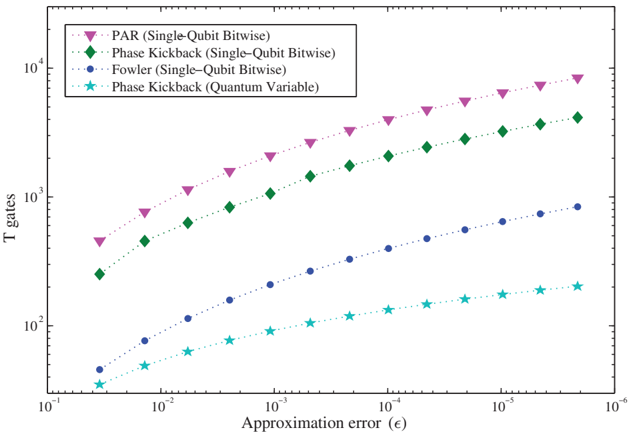
Figure 16 Number of T gates required to produce a QVR with various methods, assuming ξ = 1 and number of significant figures is chosen to satisfy the approximation error ϵ . The special-purpose 'quantum variable' phase kickback clearly requires the least circuit effort, and the asymptotic scaling of T gates is linear in log ϵ for this approach and super-quadratic for the others. The circuit depth for Fowler or phase kickback approaches is equivalent to the comparable single-qubit rotation; however, the PAR must succeed across all individual rotations for this circuit to succeed, so the mean circuit depth increases slightly. In the above, ten rounds of PAR ancilla are pre-computed for each single-qubit rotation in the QVR.
Figure 16 Number of T gates required to produce a QVR with various methods, assuming ξ = 1 and number of significant figures is chosen to satisfy the approximation error ϵ . The special-purpose 'quantum variable' phase kickback clearly requires the least circuit effort, and the asymptotic scaling of T gates is linear in log ϵ for this approach and super-quadratic for the others. The circuit depth for Fowler or phase kickback approaches is equivalent to the comparable single-qubit rotation; however, the PAR must succeed across all individual rotations for this circuit to succeed, so the mean circuit depth increases slightly. In the above, ten rounds of PAR ancilla are pre-computed for each single-qubit rotation in the QVR.CC-BY-NC-SA · From the PDF
Figure 17 Circuit depth for two instances of first-quantized simulation. The in-place calculation of potential energy computes each pairwise Coulomb interaction in sets of non-overlapping particle pairs, and both the depth and number of qubits required increase linearly with the number of particles. The fully parallel calculation creates many copies of the wavefunction to permit the potential energy to be determined in constant time, at the expense of requiring substantially more application qubits (quadratic in the number of particles). In both cases, the wavefunction precision along any spatial dimension is ten qubits, and the simulation uses 1023 time steps for 10 bits of precision, or ∼ 3 significant figures.
Figure 17 Circuit depth for two instances of first-quantized simulation. The in-place calculation of potential energy computes each pairwise Coulomb interaction in sets of non-overlapping particle pairs, and both the depth and number of qubits required increase linearly with the number of particles. The fully parallel calculation creates many copies of the wavefunction to permit the potential energy to be determined in constant time, at the expense of requiring substantially more application qubits (quadratic in the number of particles). In both cases, the wavefunction precision along any spatial dimension is ten qubits, and the simulation uses 1023 time steps for 10 bits of precision, or ∼ 3 significant figures.CC-BY-NC-SA · From the PDF
Figure 18 The efficient frontiers for various implementations of simulating LiH ground state energy on a quantum computer. Each star data point corresponds to the equivalent method in figure 12, at rotation accuracy ϵ max ⩽ 10 -4 ; similarly, first-quantized simulations use QVRs with the same accuracy. The PAR frontier (purple) and first-quantized frontier (brown) have adjustable parameters that reduce circuit depth through parallel computation at the expense of increased system size (application qubits). For example, the PAR-based algorithm only achieves the circuit depth shown in figure 12 when the system has 68 qubits, which is the yellow star here.
Figure 18 The efficient frontiers for various implementations of simulating LiH ground state energy on a quantum computer. Each star data point corresponds to the equivalent method in figure 12, at rotation accuracy ϵ max ⩽ 10 -4 ; similarly, first-quantized simulations use QVRs with the same accuracy. The PAR frontier (purple) and first-quantized frontier (brown) have adjustable parameters that reduce circuit depth through parallel computation at the expense of increased system size (application qubits). For example, the PAR-based algorithm only achieves the circuit depth shown in figure 12 when the system has 68 qubits, which is the yellow star here.CC-BY-NC-SA · From the PDF
Image 23
CC-BY-NC-SA · From the PDF

Verification

Claims the paper makes

The claims and statistics of this paper haven’t been checked yet.

Free: it reads the open-access text and checks the first 5 claims that cite a source we can check. Create a free account to check every claim.

A few free checks a day · papers already verified open instantly · results are public

Claims other papers make about this one

Each is checked against this paper’s own text: does it say what the citing paper says it does?

8 more claims about this paper

Create a free account to see every claim other papers make about this one.

See all claims — free account

Self-check

Percentages, sums and reported differences re-computed from the paper’s own numbers.

The self-check needs the paper’s full text.

Citations

Cites

Show all 99 references

Cited by

See all 149

Metadata

Authors
Cody Jones, N., Whitfield, J. D., McMahon, P. L., Yung, M.-H., Meter, R. V., Aspuru-Guzik, A., & Yamamoto, Y.
Affiliations
  • Harvard University (US)
  • Stanford University (US)
  • Keio University (JP)
  • National Institute of Informatics (JP)
Venue
New Journal of Physics
Published
2012-11-27
Volume
14
Issue
11
Pages
115023
ISSN
1367-2630 (ISSN-L)
OpenAlex
W2100129648
Cited by
145
References
97
Citations by year
2026: 8 · 2025: 6 · 2024: 12 · 2023: 9 · 2022: 10 · 2021: 5 · 2020: 11 · 2019: 14 · 2018: 15 · 2017: 4 · 2016: 11 · 2015: 15 · 2014: 12 · 2013: 10 · 2012: 3
FWCI
12.60
Type
journal article
Language
en
Open access
Licence
cc-by-nc-sa
Locations
  • New Journal of Physics (publishedVersion, cc-by-nc-sa)
  • arXiv (Cornell University) (submittedVersion)
  • Digital Access to Scholarship at Harvard (DASH) (Harvard University) (submittedVersion, cc-by)
  • DOAJ (DOAJ: Directory of Open Access Journals) (submittedVersion)
  • arXiv (Cornell University)
Funders
  • National Science Foundation (0829694, FA8721-05-C-0002, 1017244)
  • Alfred P. Sloan Foundation
  • Camille and Henry Dreyfus Foundation
  • Japan Society for the Promotion of Science
  • National Institute of Information and Communications Technology
Topics
  • Physical Sciences › Computer Science › Artificial Intelligence › Quantum Computing Algorithms and Architecture
  • Physical Sciences › Physics and Astronomy › Atomic and Molecular Physics, and Optics › Quantum Information and Cryptography
  • Physical Sciences › Physics and Astronomy › Atomic and Molecular Physics, and Optics › Quantum many-body systems
Keywords
quantum chemistry simulation, fault-tolerant quantum computing, ab initio quantum chemistry, quantum teleportation, gate construction, quantum circuit optimization, execution time

About these checks

Registry, retraction, Cites and statistics results are computed, not judged, with one exception: a printed reference that no index lists is read once by a model before it counts as a citation error. Claims are extracted by a model and kept only when their quote appears verbatim in the text; each cited source is then checked, with a model’s help, for whether it says what the claim relies on. Those verdicts can be wrong — read the claim’s quote and the cited source before relying on one.

Statistics and arithmetic are recomputed, not judged.

Confidence bands are shown only for fields calibrated on our annotated test set. None is calibrated yet, so no band is shown.

What counts as a claim ›How we measure confidence ›How we check this ›

Are you an author, or do you see a problem with this page? Request a review

How to cite

Cite CoChat for the checks on this page, and the paper for its own findings.

This page
CoChat. (2026). Citation check: Faster quantum chemistry simulation on fault-tolerant quantum computers. https://app.cochat.ai/papers/10.1088/1367-2630/14/11/115023
The paper
Cody Jones, N., Whitfield, J. D., McMahon, P. L., Yung, M.-H., Meter, R. V., Aspuru-Guzik, A., & Yamamoto, Y. (2012). Faster quantum chemistry simulation on fault-tolerant quantum computers. New Journal of Physics. https://doi.org/10.1088/1367-2630/14/11/115023

Data sources

Bibliographic data: Semantic Scholar, OpenAlex, Crossref.

Contains information from the Semantic Scholar Academic Graph Datasets, made available under the ODC Attribution License (ODC-BY 1.0).

Semantic Scholar’s data is described in: Kinney, R., et al. (2023). The Semantic Scholar Open Data Platform. arXiv:2301.10140.