

Dynamical modeling and multi-experiment fitting with PottersWheel
Open accessThe DOI matches its Crossref record; 26 of the 27 references it cites were found in a registry or an index.
Abstract
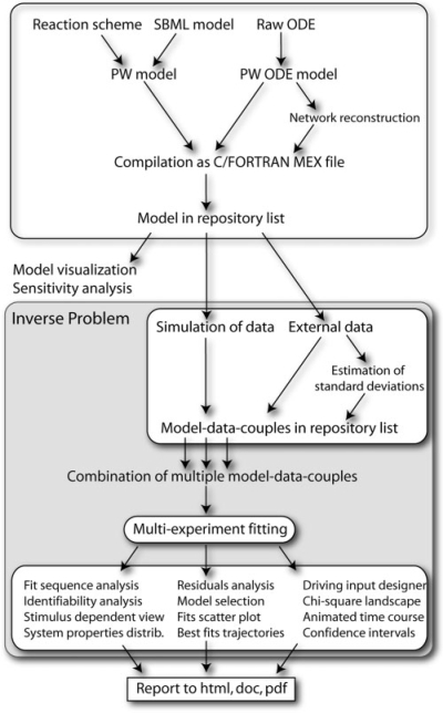
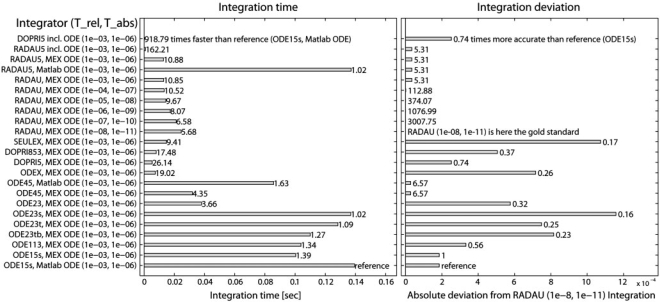
Motivation: Modelers in Systems Biology need a flexible framework that allows them to easily create new dynamic models, investigate their properties and fit several experimental datasets simultaneously. Multi-experiment-fitting is a powerful approach to estimate parameter values, to check the validity of a given model, and to discriminate competing model hypotheses. It requires high-performance integration of ordinary differential equations and robust optimization. Results: We here present the comprehensive modeling framework Potters-Wheel (PW) including novel functionalities to satisfy these requirements with strong emphasis on the inverse problem, i.e. data-based modeling of partially observed and noisy systems like signal transduction pathways and metabolic networks. PW is designed as a MATLAB toolbox and includes numerous user interfaces. Deterministic and stochastic optimization routines are combined by fitting in logarithmic parameter space allowing for robust parameter calibration. Model investigation includes statistical tests for model-data-compliance, model discrimination, identifiability analysis and calculation of Hessian- and Monte-Carlo-based parameter confidence limits. A rich application programming interface is available for customization within own MATLAB code. Within an extensive performance analysis, we identified and significantly improved an integrator–optimizer pair which decreases the fitting duration for a realistic benchmark model by a factor over 3000 compared to MATLAB with optimization toolbox. Availability: PottersWheel is freely available for academic usage at http://www.PottersWheel.de/. The website contains a detailed documentation and introductory videos. The program has been intensively used since 2005 on Windows, Linux and Macintosh computers and does not require special MATLAB toolboxes. Contact: maiwald@fdm.uni-freiburg.de Supplementary information: Supplementary data are available at Bioinformatics online.
Overview
The claims and statistics of this paper haven’t been checked yet.
Free: it reads the open-access text and checks the first 5 claims that cite a source we can check. Create a free account to check every claim.
Integrity signals
Registry
Cites
Statistics
Figures
Verification
Claims the paper makes
The claims and statistics of this paper haven’t been checked yet.
Free: it reads the open-access text and checks the first 5 claims that cite a source we can check. Create a free account to check every claim.
Claims other papers make about this one
Each is checked against this paper’s own text: does it say what the citing paper says it does?
In the citing paper
“Note that both come in forms which either incorporate information about the local geometry or not and that including such information usually leads to faster convergence [11,54].”
From Parameter uncertainty in biochemical models described by ordinary differential equations (2013) · cites this paper as [11]
In the citing paper
“For the former, model simulation time is a primary concern which can be significantly reduced by using compiled simulation code [see COPASI (Hoops et al., 2006); ABC-SysBio (Liepe et al., 2010); Potters Wheel (Maiwald and Timmer, 2008); Sloppy Cell (Brown and Sethna, 2003)].”
From A bayesian approach to targeted experiment design (2012) · cites this paper as Maiwald and Timmer, 2008
Self-check
Percentages, sums and reported differences re-computed from the paper’s own numbers.
The self-check needs the paper’s full text.
Citations
Cites
Genetic algorithms in search, optimization, and machine learning
(1989) · Choice Reviews Online · doi:10.5860/choice.27-0936 · Cited by 49,010 · cited 2×
“The simulated annealing (Ingber, 1989) and genetic algorithms (MATLAB genetic algorithm toolbox; (Goldberg, 1989)) are stochastic approaches able to handle local minima, but requiring more time.”
MethodEstimating the Dimension of a Model
Schwarz, G. (1978) · The Annals of Statistics · doi:10.1214/aos/1176344136 · Cited by 47,033 · cited 2×
“Criteria like an Information Criterion (AIC) and Bayesian information criterion (BIC) are suggested to establish a ranking of models (Akaike, 1973; Schwartz, 1978).”
BackgroundGenetic Algorithms in Search, Optimization and Machine Learning
Goldberg, D. E., & Robson, D. (1988) · Cited by 18,391
Numerical recipes in C: the art of scientific computing
(1993) · Choice Reviews Online · doi:10.5860/choice.30-5638 · Cited by 17,933
Information Theory and an Extension of the Maximum Likelihood Principle
Akaike, H. (1998) · Springer Series in Statistics · doi:10.1007/978-1-4612-1694-0_15 · Cited by 17,781
Goldberg, D. E., & Shakespeare, W. (2002) · Cited by 16,088
Convergence Properties of the Nelder--Mead Simplex Method in Low Dimensions
Lagarias, J. C., Reeds, J. A., Wright, M. H., & Wright, P. E. (1998) · SIAM Journal on Optimization · doi:10.1137/s1052623496303470 · Cited by 7,447
Inverse Problem Theory and Methods for Model Parameter Estimation
Tarantola, A. (2005) · doi:10.1137/1.9780898717921 · Cited by 6,585 · cited 1×
“PW, on the other hand, originates from the inverse problem, where for existing data a model has to be identified ((Tarantola, 2004)).”
BackgroundSolving Ordinary Differential Equations II
Hairer, E., & Wanner, G. (1996) · Springer Series in Computational Mathematics · doi:10.1007/978-3-642-05221-7 · Cited by 4,342
An Interior Trust Region Approach for Nonlinear Minimization Subject to Bounds
Coleman, T. F., & Li, Y. (1996) · SIAM Journal on Optimization · doi:10.1137/0806023 · Cited by 3,320 · cited 1×
“The trust region (MATLAB optimization toolbox; (Coleman and Li, 1996)) and Levenberg–Marquardt (Nielsen, 2006) algorithms are powerful deterministic least-square optimizers.”
MethodCOPASI—a COmplex PAthway SImulator
Hoops, S., Sahle, S., Gauges, R., Lee, C., Pahle, J., Simus, N., Singhal, M., Xu, L., Mendes, P., & Kummer, U. (2006) · Bioinformatics · doi:10.1093/bioinformatics/btl485 · Cited by 2,618
Crimins, F. (2003) · Applied Biochemistry and Biotechnology · doi:10.1007/s12010-003-0001-6 · Cited by 2,000
Testing Statistical Hypotheses
Lehmann, E. L. (1986) · Springer Texts in Statistics · doi:10.1007/978-1-4757-1923-9 · Cited by 1,873
Very fast simulated re-annealing
Ingber, L. (1989) · Mathematical and Computer Modelling · doi:10.1016/0895-7177(89)90202-1 · Cited by 1,286 · cited 1×
“If the original measurements have a non-Gaussian distributed error, they should be transformed appropriately Kreutz et al. (2007). The residual analysis of PottersWheel comprises the following graphs: 1.”
BackgroundTesting Statistical Hypothesis.
Crouse, C. F., & Lehmann, E. L. (1960) · Biometrika · doi:10.2307/2332982 · Cited by 745
Systems biology toolbox for matlab: a computational platform for research in systems biology
Schmidt, H., & Jirstrand, M. (2006) · Bioinformatics · doi:10.1093/bioinformatics/bti799 · Cited by 473 · cited 2×
“Existing modeling software like the SBToolbox (Schmidt and Jirstrand, 2006), the commercial MATLAB SymBiology toolbox, or COPASI (Hoops et al., 2006), originate from the direct problem where system properties are to be analyzed based on a given model and on parameter values.”
MethodLegewie, S., Blüthgen, N., & Herzel, H. (2006) · PLoS Computational Biology · doi:10.1371/journal.pcbi.0020120 · Cited by 241
Systems biology markup language: Level 2 and beyond
Finney, A., & Hucka, M. (2003) · Biochemical Society Transactions · doi:10.1042/bst0311472 · Cited by 187 · cited 2×
“Therefore, modeling of experimental data has been the central ∗To whom correspondence should be addressed. objective for its development from the beginning.”
BackgroundMethodPress, W. H., Teukolsky, S. A., Vettering, W. T., & Flannery, B. P. (2003) · European Journal of Physics · doi:10.1088/0143-0807/24/3/701 · Cited by 179
Data-based identifiability analysis of non-linear dynamical models
Hengl, S., Kreutz, C., Timmer, J., & Maiwald, T. (2007) · Bioinformatics · doi:10.1093/bioinformatics/btm382 · Cited by 166
Self-citationConfidence regions of estimated parameters for ecological systems
Marsili-Libelli, S., Guerrizio, S., & Checchi, N. (2003) · Ecological Modelling · doi:10.1016/s0304-3800(03)00068-1 · Cited by 92 · cited 1×
“If a Maximum Likelihood estimator is used to calibrate the parameters, the confidence intervals can be determined based on the Hessian of the objective function at the optimum ( Marsili-Libelli et al., 2003 ).”
MethodSystems biology standards—the community speaks
Klipp, E., Liebermeister, W., Helbig, A., Kowald, A., & Schaber, J. (2007) · Nature Biotechnology · doi:10.1038/nbt0407-390 · Cited by 88 · cited 1×
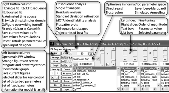
“A rich application programming interface is available for customization within own MATLAB code.”
MethodStimulus Design for Model Selection and Validation in Cell Signaling
Apgar, J. F., Toettcher, J. E., Endy, D., White, F. M., & Tidor, B. (2008) · PLoS Computational Biology · doi:10.1371/journal.pcbi.0040030 · Cited by 79
Time delay in simple chemostat models
Macdonald, N. (1976) · Biotechnology and Bioengineering · doi:10.1002/bit.260180604 · Cited by 73 · cited 2×
“Delay reactions, based on the linear chain trick (MacDonald, 1976) are important for the modeling of black box elements, e.”
BackgroundSensitivity and specificity of coherence and phase synchronization analysis
Matthias Winterhalder, A., Schelter, B. O., Kurths, J., Schulze‐Bonhage, A., & Timmer, J. (2006) · Physics Letters A · doi:10.1016/j.physleta.2006.03.018 · Cited by 37
Self-citationDynamic Pathway Modeling: Feasibility Analysis and Optimal Experimental Design
Maiwald, T., Kreutz, C., Pfeifer, A. C., Böhl, S., Klingmüller, U., & Timmer, J. (2007) · Annals of the New York Academy of Sciences · doi:10.1196/annals.1407.007 · Cited by 16
Self-citation
Research works printed but not linked: 1
- Tarantola, 2004, Inverse Problem Theory and Model Parameter Estimation.
Cited by
Raue, A., Kreutz, C., Maiwald, T., Bachmann, J., Schilling, M., Klingmüller, U., & Timmer, J. (2009) · Bioinformatics · doi:10.1093/bioinformatics/btp358 · Cited by 1,442
Self-citationEffective connectivity: Influence, causality and biophysical modeling
Valdes-Sosa, P. A., Roebroeck, A., Daunizeau, J., & Friston, K. (2011) · NeuroImage · doi:10.1016/j.neuroimage.2011.03.058 · Cited by 390
“Another framework for modeling and fitting systems defined by differential equations in bioinformatics is “Potters Wheel” (Maiwald and Timmer, 2008), which uses a profile likelihood approach (Raue et al., 2009) to explore “practical Identifiability” in addition to structural (theoretical) Identifiability.”
MethodKinetic models in industrial biotechnology – Improving cell factory performance
Almquist, J., Cvijovic, M., Hatzimanikatis, V., Nielsen, J., & Jirstrand, M. (2014) · Metabolic Engineering · doi:10.1016/j.ymben.2014.03.007 · Cited by 293
“…2006), the Systems Biology Toolbox (Schmidt and Jirstrand, 2006; Schmidt, 2007), COPASI (Hoops et al., 2006; Mendes et al., 2009), PottersWheel (Maiwald and Timmer, 2008), and AMIGO (Balsa-Canto and Banga, 2011). are several parameter sets that are equally likely to have produced the measured…”
MethodEvaluating Strategies to Normalise Biological Replicates of Western Blot Data
Degasperi, A., Birtwistle, M. R., Volinsky, N., Rauch, J., Kolch, W., & Kholodenko, B. N. (2014) · PLoS ONE · doi:10.1371/journal.pone.0087293 · Cited by 228
“In this setting, data is compared to the output of a model and appropriate values for the parameters of the model are identified, aiming to obtain the best possible agreement between data and output [4].”
BackgroundMethodProgramming biological models in Python using PySB
Lopez, C. F., Muhlich, J. L., Bachman, J. A., & Sorger, P. K. (2013) · Molecular Systems Biology · doi:10.1038/msb.2013.1 · Cited by 230
Metadata
- Authors
- Maiwald, T., & Timmer, J.
- Affiliations
- University of Freiburg (DE)
- Corresponding author
- Maiwald, Thomas
- ORCID
- Timmer, Jens
- Venue
- Bioinformatics
- Publisher
- Oxford University Press (OUP)
- Published
- 2008-07-09
- Volume
- 24
- Issue
- 18
- Pages
- 2037-2043
- ISSN
- 1367-4803 (ISSN-L)
- 1367-4811
- PMC
- PMC2530888
- OpenAlex
- W2166071821
- Cited by
- 231
- References
- 27
- Citations by year
- 2026: 1 · 2025: 1 · 2024: 2 · 2023: 4 · 2022: 8 · 2021: 25 · 2020: 7 · 2019: 10 · 2018: 9 · 2017: 13 · 2016: 14 · 2015: 16 · 2014: 17 · 2013: 19 · 2012: 30
- FWCI
- 7.55
- Type
- journal article
- Language
- en
- Open access
- hybrid
- doi.org
- Licence
- Locations
- Bioinformatics (publishedVersion, cc-by-nc)
- Europe PMC (PubMed Central) (publishedVersion, cc-by-nc)
- PubMed Central (publishedVersion, cc-by-nc)
- PubMed (publishedVersion)
- Funders
- Bundesministerium für Bildung und Forschung (0313074D)
- European Social Fund
- Topics
- Life Sciences › Biochemistry, Genetics and Molecular Biology › Molecular Biology › Gene Regulatory Network Analysis
- Life Sciences › Biochemistry, Genetics and Molecular Biology › Molecular Biology › Microbial Metabolic Engineering and Bioproduction
- Life Sciences › Biochemistry, Genetics and Molecular Biology › Molecular Biology › Bioinformatics and Genomic Networks
- Keywords
- dynamic modeling, ordinary differential equations, parameter estimation, inverse problems, model discrimination, identifiability analysis, stochastic optimization, signaling pathways, metabolic networks, MATLAB toolbox
- MeSH terms
- Computer Simulation, Programming Languages, Software, Signal Transduction, Systems Biology
About these checks
Registry, retraction, Cites and statistics results are computed, not judged, with one exception: a printed reference that no index lists is read once by a model before it counts as a citation error. Claims are extracted by a model and kept only when their quote appears verbatim in the text; each cited source is then checked, with a model’s help, for whether it says what the claim relies on. Those verdicts can be wrong — read the claim’s quote and the cited source before relying on one.
Statistics and arithmetic are recomputed, not judged.
Confidence bands are shown only for fields calibrated on our annotated test set. None is calibrated yet, so no band is shown.
What counts as a claim ›How we measure confidence ›How we check this ›
Are you an author, or do you see a problem with this page? Request a review
Data sources
Bibliographic data: Semantic Scholar, OpenAlex, Crossref.
Contains information from the Semantic Scholar Academic Graph Datasets, made available under the ODC Attribution License (ODC-BY 1.0).
Semantic Scholar’s data is described in: Kinney, R., et al. (2023). The Semantic Scholar Open Data Platform. arXiv:2301.10140.
