Cited by 236Neuroscience and Neuropharmacology ResearchNeural dynamics and brain functionFunctional Brain Connectivity Studies

The DOI matches its Crossref record; 84 of the 84 references it cites were found in a registry or an index.

Organization of the Human Inferior Parietal Lobule Based on Receptor Architectonics

Open access
Caspers, Svenja, Schleicher, Axel, Bacha-Trams, Mareike, Palomero-Gallagher, Nicola, Amunts, Katrin, Zilles, Karl·2013·Cerebral Cortex

Abstract

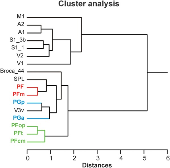
Human inferior parietal lobule (IPL) plays a key role in various cognitive functions. Its functional diversity, including attention, language, and action processing, is reflected by its structural segregation into 7 cytoarchitectonically distinct areas, each with characteristic connectivity patterns. We hypothesized that commonalities of the cytoarchitectonic, connectional, and functional diversity of the IPL should be reflected by a correlated transmitter receptor-based organization. Since the function of a cortical area requires a well-tuned receptor balance, the densities of 15 different receptors were measured in each IPL area. A hierarchical cluster analysis of the receptor balance revealed a tripartite segregation of the IPL into a rostral, middle, and caudal group. Comparison with other cortical areas showed strong similarities with Broca's region for all 3 groups, with the superior parietal cortex for the middle, and with extrastriate visual areas for the caudal group. Notably, caudal-most area PGp has a receptor fingerprint very similar to that of ventral extrastriate visual cortex. We therefore propose a new organizational model of the human IPL, consisting of 3 clusters, which corresponds to its known cytoarchitectonic, connectional, and functional diversity at the molecular level. This might reflect a general organizational principle of human IPL, beyond specific functional domains.

Overview

The claims and statistics of this paper haven’t been checked yet.

Run the check — free, no account needed. It reads the open-access text and checks the sources it cites.

A few free checks a day · papers already verified open instantly · results are public

Integrity signals

Registry

Crossref · 10.1093/cercor/bhs048

Cites

84 of 84 references verified0 citation errors · 0 not checkable

Statistics

Figures

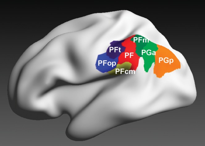
Figure 1. 3D reconstructed maximum probability maps of the 7 cytoarchitectonically defined IPL areas PFt, PFop, PF, PFm, PFcm, PGa, and PGp (Caspers et al. 2006, 2008) on the inflated lateral surface view of the Montreal Neurological Institute single subject template.
Figure 1. 3D reconstructed maximum probability maps of the 7 cytoarchitectonically defined IPL areas PFt, PFop, PF, PFm, PFcm, PGa, and PGp (Caspers et al. 2006, 2008) on the inflated lateral surface view of the Montreal Neurological Institute single subject template.CC BY-NC · PubMed Central
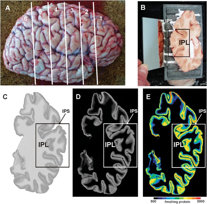
Figure 2. Quantitative in vitro receptor autoradiography. (A) Right human hemisphere prior to sectioning into 6 slabs (white lines) for further processing. (B) Blockface of a frozen slab on the cryotome with the labeled ROI in the present study (IPL). The mirror on the left side provides a lateral view of the tissue slab. (C) Autoradiograph of the GABAB receptor of the same slab, ROI marked by a box. (D) Scaled autoradiograph (same as in C) with gray values reflecting the receptor concentrations, calculated from coexposed plastic scales of known radioactivity concentrations. (E) Pseudocolor-coded autoradiograph (same as in C). The colors indicate receptor concentrations, from black for low to red for high concentrations (for concentrations in femtomole per milligram protein, see color bar). IPS: intraparietal sulcus.
Figure 2. Quantitative in vitro receptor autoradiography. (A) Right human hemisphere prior to sectioning into 6 slabs (white lines) for further processing. (B) Blockface of a frozen slab on the cryotome with the labeled ROI in the present study (IPL). The mirror on the left side provides a lateral view of the tissue slab. (C) Autoradiograph of the GABAB receptor of the same slab, ROI marked by a box. (D) Scaled autoradiograph (same as in C) with gray values reflecting the receptor concentrations, calculated from coexposed plastic scales of known radioactivity concentrations. (E) Pseudocolor-coded autoradiograph (same as in C). The colors indicate receptor concentrations, from black for low to red for high concentrations (for concentrations in femtomole per milligram protein, see color bar). IPS: intraparietal sulcus.CC BY-NC · PubMed Central
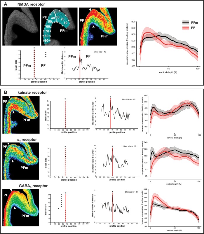
Figure 3. Parcellation of IPL based on receptor distribution patterns. (A) Part of a receptor autoradiograph (NMDA receptor) of the IPL (border region between areas PF and PFm as shown in Figure 5A for whole IPL). The autoradiograph of the cortical ribbon (upper left) was covered by traverses running perpendicular to the cortical layers (upper middle) and pseudocolor coded for visualization purposes only (upper right). Results of the algorithmic parcellation are shown below: the left graph shows the significant maxima of varying block sizes (ranging from 10 to 24); it indicates a consistently occurring border between 2 cortical areas at profile location 33. Right next to it, a line plot shows the Mahalanobis distances between neighboring blocks of profiles; it confirms the location of the maximal distance, and thus, the maximal dissimilarity between adjacent profiles at profile location 33, which defines an architectural border. The border is also labeled in the autoradiographs above. The graph on the right side of (A) shows the laminar distribution (with standard deviations) of the NMDA receptor throughout the cortical width (0% at the transition from the pial surface to layer I; 100% at the transition from layer VI to the white matter) in areas PF and PFm. The profiles differ between both areas. (B) Parcellation of the same part of the cortex by 3 other receptors (kainate, α2, and GABAB). Figures and graphs of (B) show the results of the mapping procedure comparable to (A).
Figure 3. Parcellation of IPL based on receptor distribution patterns. (A) Part of a receptor autoradiograph (NMDA receptor) of the IPL (border region between areas PF and PFm as shown in Figure 5A for whole IPL). The autoradiograph of the cortical ribbon (upper left) was covered by traverses running perpendicular to the cortical layers (upper middle) and pseudocolor coded for visualization purposes only (upper right). Results of the algorithmic parcellation are shown below: the left graph shows the significant maxima of varying block sizes (ranging from 10 to 24); it indicates a consistently occurring border between 2 cortical areas at profile location 33. Right next to it, a line plot shows the Mahalanobis distances between neighboring blocks of profiles; it confirms the location of the maximal distance, and thus, the maximal dissimilarity between adjacent profiles at profile location 33, which defines an architectural border. The border is also labeled in the autoradiographs above. The graph on the right side of (A) shows the laminar distribution (with standard deviations) of the NMDA receptor throughout the cortical width (0% at the transition from the pial surface to layer I; 100% at the transition from layer VI to the white matter) in areas PF and PFm. The profiles differ between both areas. (B) Parcellation of the same part of the cortex by 3 other receptors (kainate, α2, and GABAB). Figures and graphs of (B) show the results of the mapping procedure comparable to (A).CC BY-NC · PubMed Central
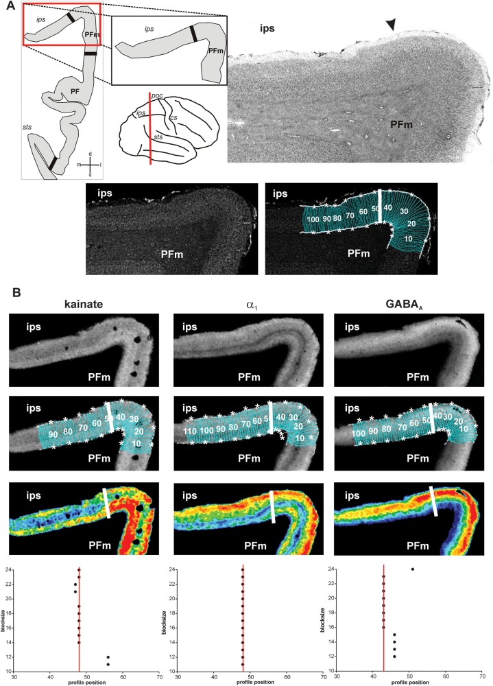
Figure 4. Algorithm-based detection of areal borders in receptor and corresponding cytoarchitectonic sections. (A) Cytoarchitectonic border between area PFm and areas within the intraparietal sulcus (IPS), sectioning level (red line), and schematic drawing of the IPL within this section with all detected borders (black thick lines) depicted on the left. Corresponding gray level index image and traverses covering the cortical ribbon beneath with detected border indicated by a white bold line at profile position no. 47. (B) Same border on corresponding sections of kainate, GABAA, and α1 receptors. For each receptor, the linearized autoradiograph, superimposed with traverses covering the ROI, and pseudocolor coded for visualization purposes. Position of the border indicated by white bold lines and in the graphs at the bottom at the respective profile position (same type of graphs as in Fig. 3). Area PFm differs from intraparietal areas by means of higher concentrations of kainate in middle and lower layers, higher concentrations of α1 in infragranular layers and of GABAA in supragranular layers. Note the close resemblance of the position of the border in cyto- and receptor sections. cs: central sulcus, ips: intraparietal sulcus, poc: postcentral sulcus, sts: superior temporal sulcus.
Figure 4. Algorithm-based detection of areal borders in receptor and corresponding cytoarchitectonic sections. (A) Cytoarchitectonic border between area PFm and areas within the intraparietal sulcus (IPS), sectioning level (red line), and schematic drawing of the IPL within this section with all detected borders (black thick lines) depicted on the left. Corresponding gray level index image and traverses covering the cortical ribbon beneath with detected border indicated by a white bold line at profile position no. 47. (B) Same border on corresponding sections of kainate, GABAA, and α1 receptors. For each receptor, the linearized autoradiograph, superimposed with traverses covering the ROI, and pseudocolor coded for visualization purposes. Position of the border indicated by white bold lines and in the graphs at the bottom at the respective profile position (same type of graphs as in Fig. 3). Area PFm differs from intraparietal areas by means of higher concentrations of kainate in middle and lower layers, higher concentrations of α1 in infragranular layers and of GABAA in supragranular layers. Note the close resemblance of the position of the border in cyto- and receptor sections. cs: central sulcus, ips: intraparietal sulcus, poc: postcentral sulcus, sts: superior temporal sulcus.CC BY-NC · PubMed Central
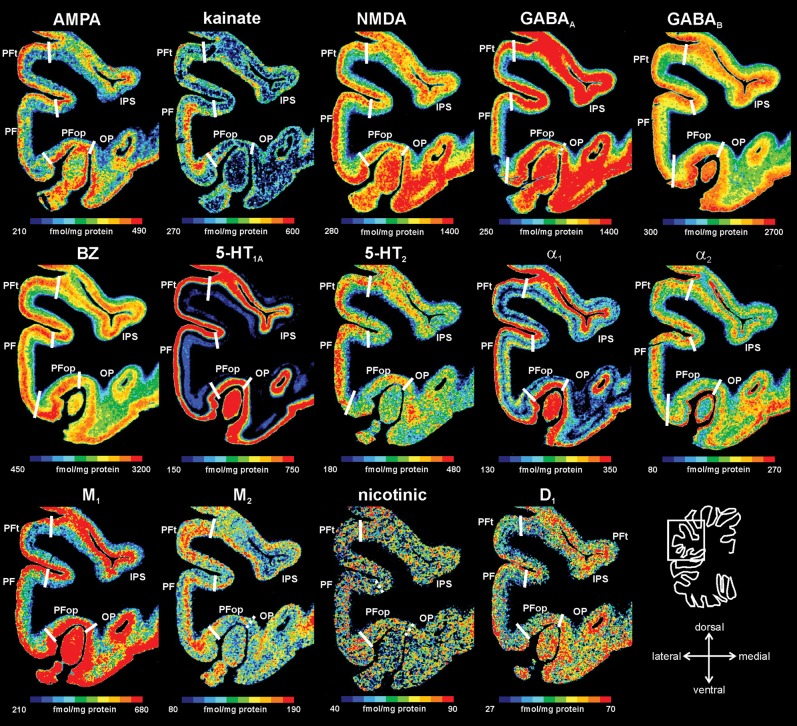
Figure 5. Receptor distribution patterns in areas PF, PFop, and PFt illustrated for 14 of the 15 receptors studied. Pseudocolor-coded autoradiographs show the borders between the IPL areas (white lines). The color bar beneath each autoradiograph indicates receptor concentrations by the different colors, from black for low to red for high concentrations (in femtomole per milligram protein). Note that the scaling is different for each receptor.
Figure 5. Receptor distribution patterns in areas PF, PFop, and PFt illustrated for 14 of the 15 receptors studied. Pseudocolor-coded autoradiographs show the borders between the IPL areas (white lines). The color bar beneath each autoradiograph indicates receptor concentrations by the different colors, from black for low to red for high concentrations (in femtomole per milligram protein). Note that the scaling is different for each receptor.CC BY-NC · PubMed Central
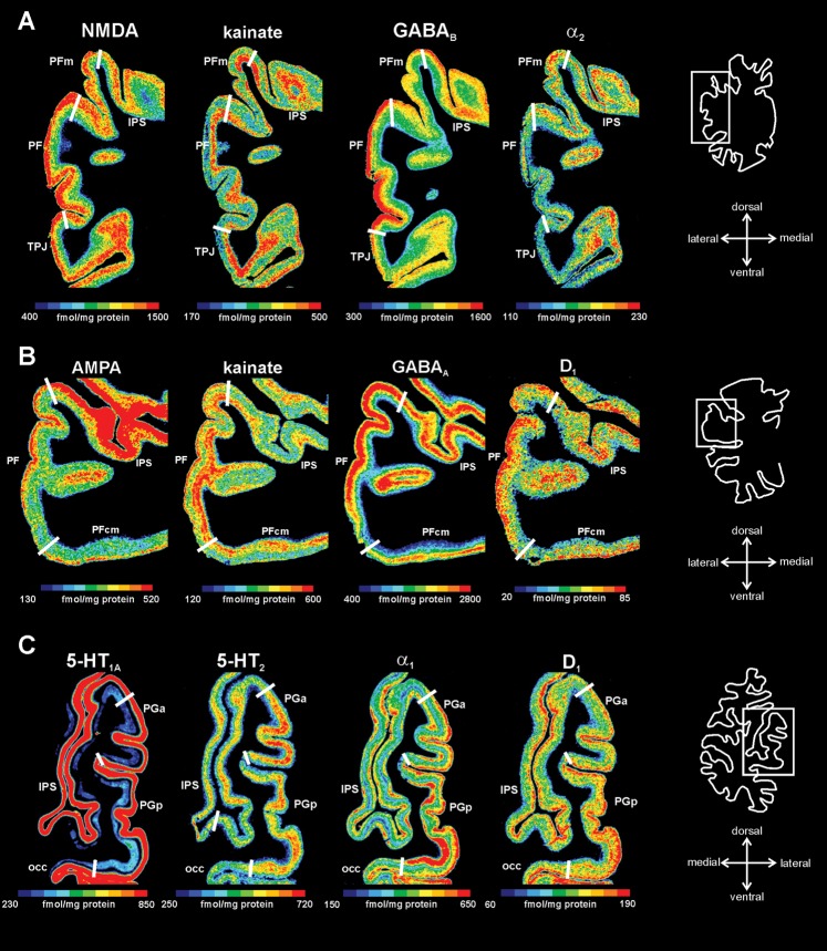
Figure 6. Receptor distribution patterns of areas PF, PFm, PFcm, PGa, and PGp for those receptors, which showed most prominent differences between the areas. (A) Delineation of areas PF and PFm (same level as in Fig. 3). (B) Delineation of areas PF and PFcm. (C) Delineation of areas PGa and PGp. For other conventions, see Figure 4.
Figure 6. Receptor distribution patterns of areas PF, PFm, PFcm, PGa, and PGp for those receptors, which showed most prominent differences between the areas. (A) Delineation of areas PF and PFm (same level as in Fig. 3). (B) Delineation of areas PF and PFcm. (C) Delineation of areas PGa and PGp. For other conventions, see Figure 4.CC BY-NC · PubMed Central
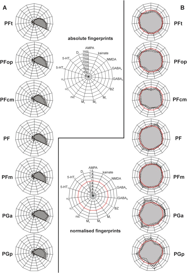
Figure 7. Receptor fingerprints of the 7 IPL areas PFt, PFop, PF, PFm, PFcm, PGa, and PGp. (A) Polar plots (scaling 0–3500 femtomole per milligram protein) showing the mean (averaged over all cortical layers) absolute receptor concentrations of all 15 receptors (with standard error of the mean as dotted lines) of each area. (B) Polar plots (scaling 0–1.6) showing the normalized receptor concentration of all 15 receptors (with standard error of the mean as dotted lines). Normalization of the receptor concentrations was calculated based on each receptor's mean over the whole IPL. Red thick line indicates the 100% line (labeled 1) where the receptor concentration of an area was equal to the mean receptor concentration averaged over the whole IPL. Note the difference in size and shape between the fingerprints of the different areas.
Figure 7. Receptor fingerprints of the 7 IPL areas PFt, PFop, PF, PFm, PFcm, PGa, and PGp. (A) Polar plots (scaling 0–3500 femtomole per milligram protein) showing the mean (averaged over all cortical layers) absolute receptor concentrations of all 15 receptors (with standard error of the mean as dotted lines) of each area. (B) Polar plots (scaling 0–1.6) showing the normalized receptor concentration of all 15 receptors (with standard error of the mean as dotted lines). Normalization of the receptor concentrations was calculated based on each receptor's mean over the whole IPL. Red thick line indicates the 100% line (labeled 1) where the receptor concentration of an area was equal to the mean receptor concentration averaged over the whole IPL. Note the difference in size and shape between the fingerprints of the different areas.CC BY-NC · PubMed Central
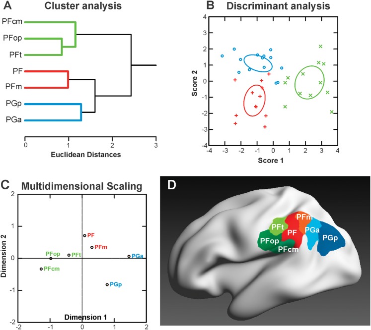
Figure 8. Segregation of IPL areas based on multiple receptor densities averaged over all cortical layers. (A) Hierarchical cluster analysis reveals 3 receptor-architectonically distinct clusters: a rostral cluster with areas PFop, PFt, PFcm (green), an intermediate cluster with areas PF and PFm (red), and a caudal cluster with areas PGa and PGp (blue). (B) Canonical discriminant analysis of all available receptor data in IPL. For each of the 3 clusters, the n data points (n = number of areas in that cluster × number of hemispheres, some points are missing due to missing values for some receptor types) are indicated by different symbols. Ellipses provide the 90% confidence interval of the centroids. Same color coding as in (A). (C) MDS analysis visualizes the differences between the 3 clusters. Same color coding as in (A). (D) Visualization of the resulting 3 clusters within the IPL, using the same depiction of the cytoarchitectonically defined IPL areas (Caspers et al. 2006, 2008) as in Figure 1. Color coding of the areas corresponding to the receptor-based cluster segregation: rostral cluster (areas PFt, PFop, and PFcm): shades of green; middle cluster (areas PF and PFm): shades of red; caudal cluster (areas PGa and PGp): shades of blue.
Figure 8. Segregation of IPL areas based on multiple receptor densities averaged over all cortical layers. (A) Hierarchical cluster analysis reveals 3 receptor-architectonically distinct clusters: a rostral cluster with areas PFop, PFt, PFcm (green), an intermediate cluster with areas PF and PFm (red), and a caudal cluster with areas PGa and PGp (blue). (B) Canonical discriminant analysis of all available receptor data in IPL. For each of the 3 clusters, the n data points (n = number of areas in that cluster × number of hemispheres, some points are missing due to missing values for some receptor types) are indicated by different symbols. Ellipses provide the 90% confidence interval of the centroids. Same color coding as in (A). (C) MDS analysis visualizes the differences between the 3 clusters. Same color coding as in (A). (D) Visualization of the resulting 3 clusters within the IPL, using the same depiction of the cytoarchitectonically defined IPL areas (Caspers et al. 2006, 2008) as in Figure 1. Color coding of the areas corresponding to the receptor-based cluster segregation: rostral cluster (areas PFt, PFop, and PFcm): shades of green; middle cluster (areas PF and PFm): shades of red; caudal cluster (areas PGa and PGp): shades of blue.CC BY-NC · PubMed Central
Figure 9. Receptor distributions of IPL areas compared with those of other cortical areas. The hierarchical cluster analysis that shows the same tripartition of the IPL areas as shown in Figure 8 but additionally reveals similarities of the intermediate cluster (areas PF and PFm, red) with superior parietal areas (SPLs) and of the caudal cluster (areas PGa and PGp, blue) with extrastriate visual areas. The IPL areas are most similar to each other and similar to higher order areas (Broca_44, SPL, and V3v) but are most dissimilar to primary and secondary areas (A1/A2, M1, S1, and V1/V2). Note the close resemblance of area PGp with extrastriate visual area V3v. A1/A2: primary/secondary auditory cortex, Broca_44: area 44 of Broca's region, M1: primary motor cortex, S1_3b: area 3b of primary somatosensory cortex, S1_1: area 1 of primary somatosensory cortex, SPL: superior parietal lobule, V1/V2: primary/secondary visual cortex, V3v: ventral extrastriate visual cortex.
Figure 9. Receptor distributions of IPL areas compared with those of other cortical areas. The hierarchical cluster analysis that shows the same tripartition of the IPL areas as shown in Figure 8 but additionally reveals similarities of the intermediate cluster (areas PF and PFm, red) with superior parietal areas (SPLs) and of the caudal cluster (areas PGa and PGp, blue) with extrastriate visual areas. The IPL areas are most similar to each other and similar to higher order areas (Broca_44, SPL, and V3v) but are most dissimilar to primary and secondary areas (A1/A2, M1, S1, and V1/V2). Note the close resemblance of area PGp with extrastriate visual area V3v. A1/A2: primary/secondary auditory cortex, Broca_44: area 44 of Broca's region, M1: primary motor cortex, S1_3b: area 3b of primary somatosensory cortex, S1_1: area 1 of primary somatosensory cortex, SPL: superior parietal lobule, V1/V2: primary/secondary visual cortex, V3v: ventral extrastriate visual cortex.CC BY-NC · PubMed Central

Verification

Claims the paper makes

The claims and statistics of this paper haven’t been checked yet.

Run the check — free, no account needed. It reads the open-access text and checks the sources it cites.

A few free checks a day · papers already verified open instantly · results are public

Self-check

Percentages, sums and reported differences re-computed from the paper’s own numbers.

The self-check needs the paper’s full text.

Citations

Cites

Show all 84 references

Cited by

Sorted by citations

See all 236

Metadata

Authors
Caspers, S., Schleicher, A., Bacha-Trams, M., Palomero-Gallagher, N., Amunts, K., & Zilles, K.
Affiliations
  • Forschungszentrum Jülich (DE)
  • Heinrich Heine University Düsseldorf (DE)
Corresponding author
Caspers, Svenja
Venue
Cerebral Cortex
Published
2012-02-28
Volume
23
Issue
3
Pages
615-628
ISSN
  • 1047-3211 (ISSN-L)
  • 1460-2199
OpenAlex
W2099052030
Cited by
236
References
84
Citations by year
2026: 9 · 2025: 16 · 2024: 13 · 2023: 16 · 2022: 24 · 2021: 13 · 2020: 13 · 2019: 13 · 2018: 21 · 2017: 26 · 2016: 21 · 2015: 21 · 2014: 10 · 2013: 13 · 2012: 6
FWCI
6.59
Type
journal article
Language
en
Open access
Licence
cc-by-nc
Locations
  • Cerebral Cortex (publishedVersion, cc-by-nc)
  • Europe PMC (PubMed Central) (publishedVersion, cc-by-nc)
  • PubMed Central (publishedVersion, cc-by-nc)
  • PubMed (publishedVersion)
  • MPG.PuRe (Max Planck Society) (submittedVersion, other-oa)
  • Max Planck Digital Library (submittedVersion, other-oa)
  • JuSER (Forschungszentrum Jülich) (submittedVersion, other-oa)
  • RWTH Publications (RWTH Aachen) (submittedVersion)
Topics
  • Life Sciences › Neuroscience › Cellular and Molecular Neuroscience › Neuroscience and Neuropharmacology Research
  • Life Sciences › Neuroscience › Cognitive Neuroscience › Neural dynamics and brain function
  • Life Sciences › Neuroscience › Cognitive Neuroscience › Functional Brain Connectivity Studies
Keywords
inferior parietal lobule, receptor structure, neurotransmitter receptors, cytoarchitecture, cortical organization, Broca's area, superior parietal cortex, extrastriate cortex, posterior parietal cortex, functional segregation
MeSH terms
Aged, Autoradiography, Brain Mapping, Female, Humans, Male, Parietal Lobe, Cluster Analysis, Receptors, Neurotransmitter

About these checks

Registry, retraction, Cites and statistics results are computed, not judged, with one exception: a printed reference that no index lists is read once by a model before it counts as a citation error. Claims are extracted by a model and kept only when their quote appears verbatim in the text; each cited source is then checked, with a model’s help, for whether it says what the claim relies on. Those verdicts can be wrong — read the claim’s quote and the cited source before relying on one.

Statistics and arithmetic are recomputed, not judged.

Confidence bands are shown only for fields calibrated on our annotated test set. None is calibrated yet, so no band is shown.

What counts as a claim ›How we measure confidence ›How we check this ›

Are you an author, or do you see a problem with this page? Request a review