

The DOI matches its Crossref record; 82 of the 83 references it cites were found in a registry or an index.
Could a Neuroscientist Understand a Microprocessor?
Open accessAbstract
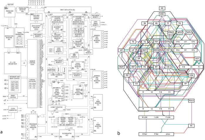
There is a popular belief in neuroscience that we are primarily data limited, and that producing large, multimodal, and complex datasets will, with the help of advanced data analysis algorithms, lead to fundamental insights into the way the brain processes information. These datasets do not yet exist, and if they did we would have no way of evaluating whether or not the algorithmically-generated insights were sufficient or even correct. To address this, here we take a classical microprocessor as a model organism, and use our ability to perform arbitrary experiments on it to see if popular data analysis methods from neuroscience can elucidate the way it processes information. Microprocessors are among those artificial information processing systems that are both complex and that we understand at all levels, from the overall logical flow, via logical gates, to the dynamics of transistors. We show that the approaches reveal interesting structure in the data but do not meaningfully describe the hierarchy of information processing in the microprocessor. This suggests current analytic approaches in neuroscience may fall short of producing meaningful understanding of neural systems, regardless of the amount of data. Additionally, we argue for scientists using complex non-linear dynamical systems with known ground truth, such as the microprocessor as a validation platform for time-series and structure discovery methods. Author Summary: Neuroscience is held back by the fact that it is hard to evaluate if a conclusion is correct; the complexity of the systems under study and their experimental inaccessability make the assessment of algorithmic and data analytic technqiues challenging at best. We thus argue for testing approaches using known artifacts, where the correct interpretation is known. Here we present a microprocessor platform as one such test case. We find that many approaches in neuroscience, when used na•vely, fall short of producing a meaningful understanding.
Overview
The claims and statistics of this paper haven’t been checked yet.
Run the check — free, no account needed. It reads the open-access text and checks the sources it cites.
Integrity signals
Registry
Cites
Statistics
Figures
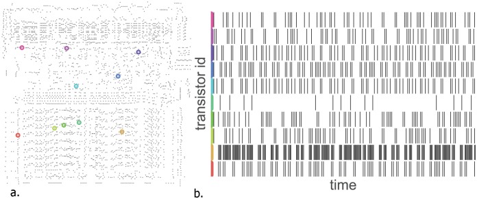
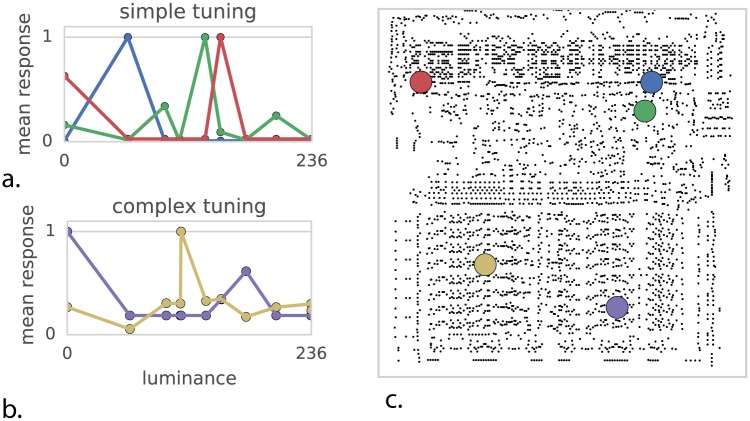
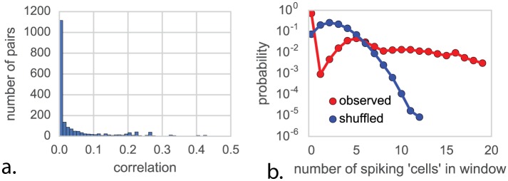
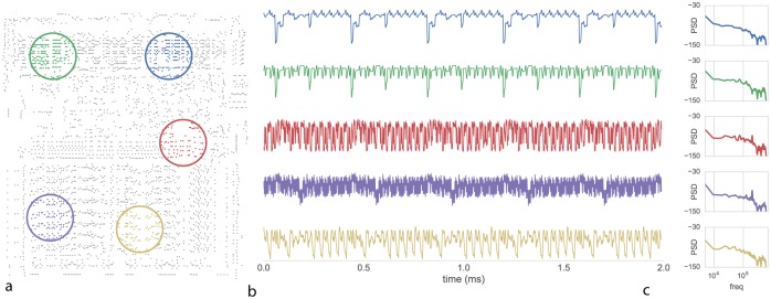
Verification
Claims the paper makes
The claims and statistics of this paper haven’t been checked yet.
Run the check — free, no account needed. It reads the open-access text and checks the sources it cites.
Claims other papers make about this one
Each is checked against this paper’s own text: does it say what the citing paper says it does?
In the citing paper
“The sobering result was that performing interventionist neuroscience on the processor could not explain how the processor worked.”
From Neuroscience Needs Behavior: Correcting a Reductionist Bias (2017) · cites this paper as Jonas and Kording, 2017
In the citing paper
“The result was that none of these techniques came close to reverse engineering the standard stored-program computer architecture”
From Neuroscience Needs Behavior: Correcting a Reductionist Bias (2017) · cites this paper as Jonas and Kording, 2017
In the citing paper
“the recent study by Jonas and Kording (Jonas and Kording, 2017) we referred to earlier provides an empirical demonstration of the fundamental difference between intervening and recording versus understanding how information flows through processing steps.”
From Neuroscience Needs Behavior: Correcting a Reductionist Bias (2017) · cites this paper as Jonas and Kording, 2017
In the citing paper
“The behavioral data analyzed consisted of 10 s of spontaneous activity with no player actually playing the game”
From Neuroscience Needs Behavior: Correcting a Reductionist Bias (2017) · cites this paper as Jonas and Kording, 2017
In the citing paper
“Due to the complexity and variability of the brain, pure “bottom up” analysis of neural data faces potential challenges of interpretation (Robinson, 1992; Jonas and Kording, 2016).”
From Toward an integration of deep learning and neuroscience (2016) · cites this paper as Jonas and Kording, 2016
Self-check
Percentages, sums and reported differences re-computed from the paper’s own numbers.
The self-check needs the paper’s full text.
Citations
Cites
Scikit-learn: Machine Learning in Python
Pedregosa, F., Varoquaux, G., Gramfort, A., Michel, V., Thirion, B., Grisel, O., Blondel, M., Müller, A., Nothman, J., Louppe, G., et al. (2012) · arXiv · doi:10.48550/arxiv.1201.0490 · Cited by 71,016
Human-level control through deep reinforcement learning
Mnih, V., Kavukcuoglu, K., Silver, D., Rusu, A. A., Veness, J., Bellemare, M. G., Graves, A., Riedmiller, M., Fidjeland, A. K., Ostrovski, G., et al. (2015) · Nature · doi:10.1038/nature14236 · Cited by 30,357
Advances in neural information processing systems 7
Cios, K. J., & Shields, M. E. (1997) · Neurocomputing · doi:10.1016/s0925-2312(97)90018-7 · Cited by 22,093
Visualizing and understanding convolutional networks
Zeiler, M. D., & Fergus, R. (2014) · Lecture Notes in Computer Science · doi:10.1007/978-3-319-10590-1_53 · Cited by 15,839
Learning the parts of objects by non-negative matrix factorization
Lee, D. D., & Seung, H. S. (1999) · Nature · doi:10.1038/44565 · Cited by 14,193
Receptive fields, binocular interaction and functional architecture in the cat’s visual cortex
Hubel, D. H., & Wiesel, T. N. (1962) · The Journal of Physiology · doi:10.1113/jphysiol.1962.sp006837 · Cited by 13,680
Intriguing properties of neural networks
Szegedy, C., Zaremba, W., Sutskever, I., Bruna, J., Erhan, D., Goodfellow, I., & Fergus, R. (2013) · arXiv · doi:10.48550/arxiv.1312.6199 · Cited by 8,143
Distributed hierarchical processing in the primate cerebral cortex
Felleman, D. J., & Van Essen, D. C. (1991) · Cerebral Cortex · doi:10.1093/cercor/1.1.1 · Cited by 7,783
The fusiform face area: a module in human extrastriate cortex specialized for face perception
Kanwisher, N., McDermott, J., & Chun, M. M. (1997) · The Journal of Neuroscience · doi:10.1523/jneurosci.17-11-04302.1997 · Cited by 7,738
Neuronal Oscillations in Cortical Networks
Buzsáki, G., & Draguhn, A. (2004) · Science · doi:10.1126/science.1099745 · Cited by 6,576
Cited by
Sorted by citations
Neuroscience-Inspired Artificial Intelligence
Hassabis, D., Kumaran, D., Summerfield, C., & Botvinick, M. (2017) · Neuron · doi:10.1016/j.neuron.2017.06.011 · Cited by 1,557
Neuroscience Needs Behavior: Correcting a Reductionist Bias
Krakauer, J. W., Ghazanfar, A. A., Gomez-Marin, A., MacIver, M. A., & Poeppel, D. (2017) · Neuron · doi:10.1016/j.neuron.2016.12.041 · Cited by 1,358
Thalamic functions in distributed cognitive control
Halassa, M. M., & Kästner, S. (2017) · Nature Neuroscience · doi:10.1038/s41593-017-0020-1 · Cited by 540
Neural Entrainment and Attentional Selection in the Listening Brain
Obleser, J., & Kayser, C. (2019) · Trends in Cognitive Sciences · doi:10.1016/j.tics.2019.08.004 · Cited by 421
Direct Fit to Nature: An Evolutionary Perspective on Biological and Artificial Neural Networks
Hasson, U., Nastase, S. A., & Goldstein, A. (2020) · Neuron · doi:10.1016/j.neuron.2019.12.002 · Cited by 387
The Border Between Seeing and Thinking
Block, N. (2023) · doi:10.1093/oso/9780197622223.001.0001 · Cited by 367
Causal mapping of human brain function
Siddiqi, S., Kording, K. P., Parvizi, J., & Fox, M. (2022) · Nature reviews. Neuroscience · doi:10.1038/s41583-022-00583-8 · Cited by 368
Diedrichsen, J., & Kriegeskorte, N. (2017) · PLoS Computational Biology · doi:10.1371/journal.pcbi.1005508 · Cited by 350
Lack of theory building and testing impedes progress in the factor and network literature
Fried, E. I. (2020) · Psychological Inquiry · doi:10.1080/1047840x.2020.1853461 · Cited by 317
Williams, A. H., Kim, T. H., Wang, F. L., Vyas, S., Ryu, S. I., Shenoy, K. V., Schnitzer, M. J., Kolda, T. G., & Ganguli, S. (2018) · Neuron · doi:10.1016/j.neuron.2018.05.015 · Cited by 320
Optimising network modelling methods for fMRI
Pervaiz, U., Vidaurre, D., Woolrich, M. W., & Smith, S. M. (2020) · NeuroImage · doi:10.1016/j.neuroimage.2020.116604 · Cited by 236
Are We Ready for Real-world Neuroscience?
Matusz, P. J., Dikker, S., Huth, A. G., & Perrodin, C. (2018) · Journal of Cognitive Neuroscience · doi:10.1162/jocn_e_01276 · Cited by 220
Representation, Pattern Information, and Brain Signatures: From Neurons to Neuroimaging
Kragel, P. A., Koban, L., Barrett, L. F., & Wager, T. D. (2018) · Neuron · doi:10.1016/j.neuron.2018.06.009 · Cited by 212
Michaels, J. A., Dann, B., & Scherberger, H. (2016) · PLoS Computational Biology · doi:10.1371/journal.pcbi.1005175 · Cited by 184
A Student’s Guide to Neural Circuit Tracing
Saleeba, C., Dempsey, B., Le, S., Goodchild, A., & McMullan, S. (2019) · Frontiers in Neuroscience · doi:10.3389/fnins.2019.00897 · Cited by 153
The roles of supervised machine learning in systems neuroscience
Glaser, J. I., Benjamin, A. S., Farhoodi, R., & Kording, K. P. (2019) · Progress in Neurobiology · doi:10.1016/j.pneurobio.2019.01.008 · Cited by 163
Big data and the industrialization of neuroscience: A safe roadmap for understanding the brain?
Frégnac, Y. (2017) · Science · doi:10.1126/science.aan8866 · Cited by 152
The Neural Code for Pain: From Single-Cell Electrophysiology to the Dynamic Pain Connectome
Kucyi, A., & Davis, K. D. (2016) · The Neuroscientist · doi:10.1177/1073858416667716 · Cited by 152
Engemann, D. A., Kozynets, O., Sabbagh, D., Lemaitre, G., Varoquaux, G. P., Liem, F., & Gramfort, A. (2020) · eLife · doi:10.7554/elife.54055 · Cited by 142
Symmetry Breaking in Space-Time Hierarchies Shapes Brain Dynamics and Behavior
Pillai, A. S., & Jirsa, V. (2017) · Neuron · doi:10.1016/j.neuron.2017.05.013 · Cited by 132
Investigating Emotions as Functional States Distinct From Feelings
Adolphs, R., & Andler, D. (2018) · Emotion Review · doi:10.1177/1754073918765662 · Cited by 126
Toward an integration of deep learning and neuroscience
Marblestone, A. H., Wayne, G., & Kording, K. P. (2016) · Frontiers in Computational Neuroscience · doi:10.3389/fncom.2016.00094 · Cited by 119
Bongard, J., & Levin, M. G. (2021) · Frontiers in Ecology and Evolution · doi:10.3389/fevo.2021.650726 · Cited by 132
Quasi-experimental causality in neuroscience and behavioural research
Marinescu, I., Lawlor, P. N., & Kording, K. P. (2018) · Nature Human Behaviour · doi:10.1038/s41562-018-0466-5 · Cited by 107
A perspective on cortical layering and layer-spanning neuronal elements
Larkum, M. E., Petro, L. S., Sachdev, R. N. S., & Muckli, L. (2018) · Frontiers in Neuroanatomy · doi:10.3389/fnana.2018.00056 · Cited by 102
Internal model recalibration does not deteriorate with age while motor adaptation does
Vandevoorde, K., & de Xivry, J. O. (2019) · Neurobiology of Aging · doi:10.1016/j.neurobiolaging.2019.03.020 · Cited by 105
Colombo, M., & Piccinini, G. (2023) · doi:10.1017/9781009183734 · Cited by 106
Recovering Within-Person Dynamics from Psychological Time Series
Haslbeck, J. M. B., & Ryan, O. (2021) · Multivariate Behavioral Research · doi:10.1080/00273171.2021.1896353 · Cited by 101
The sociology of scientific validity: How professional networks shape judgement in peer review
Teplitskiy, M., Acuna, D., Elamrani-Raoult, A., Körding, K., & Evans, J. (2018) · Research Policy · doi:10.1016/j.respol.2018.06.014 · Cited by 113
Neural data science: accelerating the experiment-analysis-theory cycle in large-scale neuroscience
Paninski, L., & Cunningham, J. (2018) · Current Opinion in Neurobiology · doi:10.1016/j.conb.2018.04.007 · Cited by 100
Basal Ganglia Circuits for Action Specification
Park, J., Coddington, L. T., & Dudman, J. T. (2020) · Annual Review of Neuroscience · doi:10.1146/annurev-neuro-070918-050452 · Cited by 96
On Logical Inference over Brains, Behaviour, and Artificial Neural Networks
Guest, O., & Martin, A. E. (2023) · Computational Brain & Behavior · doi:10.1007/s42113-022-00166-x · Cited by 96
Functional neuroimaging in psychiatry and the case for failing better
Nour, M. M., Liu, Y., & Dolan, R. J. (2022) · Neuron · doi:10.1016/j.neuron.2022.07.005 · Cited by 92
Towards algorithmic analytics for large-scale datasets
Bzdok, D., Nichols, T. E., & Smith, S. M. (2019) · Nature Machine Intelligence · doi:10.1038/s42256-019-0069-5 · Cited by 89
Are Dendrites Conceptually Useful?
Larkum, M. E. (2022) · Neuroscience · doi:10.1016/j.neuroscience.2022.03.008 · Cited by 84
Chirimuuta, M. (2024) · The MIT Press eBooks · doi:10.7551/mitpress/13804.001.0001 · Cited by 82
Clawson, W. P., & Levin, M. G. (2022) · Biological Journal of the Linnean Society · doi:10.1093/biolinnean/blac073 · Cited by 76
Toward a neuroscience of natural behavior
Cisek, P., & Green, A. M. (2024) · Current Opinion in Neurobiology · doi:10.1016/j.conb.2024.102859 · Cited by 97
Inference in the Brain: Statistics Flowing in Redundant Population Codes
Pitkow, X., & Angelaki, D. E. (2017) · Neuron · doi:10.1016/j.neuron.2017.05.028 · Cited by 79
Computational Foundations of Natural Intelligence
van Gerven, M. A. J. (2017) · Frontiers in Computational Neuroscience · doi:10.3389/fncom.2017.00112 · Cited by 76
Degeneracy in hippocampal physiology and plasticity
Rathour, R. K., & Narayanan, R. (2019) · Hippocampus · doi:10.1002/hipo.23139 · Cited by 78
Predictive coding and stochastic resonance as fundamental principles of auditory phantom perception.
Schilling, A., Sedley, W., Gerum, R., Metzner, C., Tziridis, K., Maier, A., Schulze, H., Zeng, F.-G., Friston, K. J., & Krauss, P. (2023) · Brain · doi:10.1093/brain/awad255 · Cited by 70
Hagendorff, T., Dasgupta, I., Binz, M., Chan, S. C. Y., Lampinen, A., Wang, J. X., Akata, Z., & Schulz, E. (2023) · arXiv · doi:10.48550/arxiv.2303.13988 · Cited by 68
Blindness and Human Brain Plasticity
Fine, I., & Park, J.-M. (2018) · Annual Review of Vision Science · doi:10.1146/annurev-vision-102016-061241 · Cited by 72
Khambhati, A. N., Kahn, A. E., Costantini, J. G., Ezzyat, Y., Solomon, E. A., Gross, R. E., Jobst, B. C., Sheth, S. A., Zaghloul, K. A., Worrell, G. A., et al. (2019) · Network Neuroscience · doi:10.1162/netn_a_00089 · Cited by 62
Predicting degradation rate of genipin cross-linked gelatin scaffolds with machine learning
Entekhabi, E., Nazarpak, M. H., Sedighi, M., & Kazemzadeh, A. (2019) · Materials Science and Engineering C · doi:10.1016/j.msec.2019.110362 · Cited by 63
Diedrichsen, J., Yokoi, A., & Arbuckle, S. A. (2017) · NeuroImage · doi:10.1016/j.neuroimage.2017.08.051 · Cited by 61
Performance reserves in brain-imaging-based phenotype prediction
Schulz, M.-A., Bzdok, D., Haufe, S., Haynes, J., & Ritter, K. (2023) · Cell Reports · doi:10.1016/j.celrep.2023.113597 · Cited by 62
Probabilistic language models in cognitive neuroscience: Promises and pitfalls
Armeni, K., Willems, R. M., & Frank, S. L. (2017) · Neuroscience & Biobehavioral Reviews · doi:10.1016/j.neubiorev.2017.09.001 · Cited by 61
Frequency Selectivity of Persistent Cortical Oscillatory Responses to Auditory Rhythmic Stimulation
Lerousseau, J. P., Trébuchon, A., Morillon, B., & Schön, D. (2021) · Journal of Neuroscience · doi:10.1523/jneurosci.0213-21.2021 · Cited by 62
Danchin, A., Ouzounis, C., Tokuyasu, T., & Zucker, J. (2018) · Microbial Biotechnology · doi:10.1111/1751-7915.13284 · Cited by 56
Infrastructural intelligence: Contemporary entanglements between neuroscience and AI
Bruder, J. (2017) · Progress in brain research · doi:10.1016/bs.pbr.2017.06.004 · Cited by 58
Can Computers Become Conscious and Overcome Humans?
Signorelli, C. M. (2018) · Frontiers in Robotics and AI · doi:10.3389/frobt.2018.00121 · Cited by 64
Sparsity through evolutionary pruning prevents neuronal networks from overfitting
Gerum, R. C., Erpenbeck, A., Krauß, P., & Schilling, A. (2020) · Neural Networks · doi:10.1016/j.neunet.2020.05.007 · Cited by 56
Lack of theory building and testing impedes progress in the factor and network literaturePreprint
Fried, E. I. (2020) · PsyArXiv (OSF Preprints) · doi:10.31234/osf.io/zg84s · Cited by 78
The dynamical renaissance in neuroscience
Favela, L. H. (2020) · Synthese · doi:10.1007/s11229-020-02874-y · Cited by 55
The Neuroscience of Spatial Navigation and the Relationship to Artificial Intelligence
Bermudez-Contreras, E. J., Clark, B. J., & Wilber, A. A. (2020) · Frontiers in Computational Neuroscience · doi:10.3389/fncom.2020.00063 · Cited by 54
Cockrell, C., & An, G. C. (2017) · Journal of Theoretical Biology · doi:10.1016/j.jtbi.2017.07.016 · Cited by 50
An Algorithmic Approach to Natural Behavior
Hein, A. M., Altshuler, D. L., Cade, D. E., Liao, J. C., Martin, B. T., & Taylor, G. K. (2020) · Current Biology · doi:10.1016/j.cub.2020.04.018 · Cited by 54
A call for more clarity around causality in neuroscience
Barack, D. L., Miller, E. K., Moore, C. I., Packer, A. M., Pessoa, L., Ross, L. N., & Rust, N. C. (2022) · Trends in Neurosciences · doi:10.1016/j.tins.2022.06.003 · Cited by 48
Dentate spikes and external control of hippocampal function
Dvořák, D., Chung, A., Park, E., & Fenton, A. A. (2021) · Cell Reports · doi:10.1016/j.celrep.2021.109497 · Cited by 49
Blazed oblique plane microscopy reveals scale-invariant inference of brain-wide population activity
Hoffmann, M., Henninger, J., Veith, J., Richter, L., & Judkewitz, B. (2023) · Nature Communications · doi:10.1038/s41467-023-43741-x · Cited by 48
Stocco, A., Sibert, C., Steine-Hanson, Z., Koh, N., Laird, J. E., Lebiere, C. J., & Rosenbloom, P. S. (2021) · NeuroImage · doi:10.1016/j.neuroimage.2021.118035 · Cited by 52
Deep neuroethology of a virtual rodent
Merel, J., Aldarondo, D., Marshall, J., Tassa, Y., Wayne, G., & Ölveczky, B. (2019) · arXiv · doi:10.48550/arxiv.1911.09451 · Cited by 44
The use of artificial media in fungal ecology
Crowther, T. W., Boddy, L., & Maynard, D. S. (2017) · Fungal ecology · doi:10.1016/j.funeco.2017.10.007 · Cited by 43
Chronic pain as embodied defence: implications for current and future psychological treatments
Eccleston, C. (2018) · Pain · doi:10.1097/j.pain.0000000000001286 · Cited by 43
A quantitative model of conserved macroscopic dynamics predicts future motor commands
Brennan, C. M., & Proekt, A. (2019) · eLife · doi:10.7554/elife.46814 · Cited by 45
Oathes, D. J., Balderston, N. L., Kording, K. P., Deluisi, J. A., Perez, G. M., Medaglia, J. D., Yong Fan, A., Duprat, R., Satterthwaite, T. D., Sheline, Y. I., et al. (2021) · Wiley Interdisciplinary Reviews Cognitive Science · doi:10.1002/wcs.1553 · Cited by 43
Berger, S., & Baria, A. T. (2022) · Frontiers in Pain Research · doi:10.3389/fpain.2022.896276 · Cited by 42
Navlakha, S., Bar‐Joseph, Z., & Barth, A. L. (2017) · Trends in Cognitive Sciences · doi:10.1016/j.tics.2017.09.012 · Cited by 43
On neuromechanical approaches for the study of biological and robotic grasp and manipulation
Valero‐Cuevas, F. J., & Santello, M. (2017) · Journal of NeuroEngineering and Rehabilitation · doi:10.1186/s12984-017-0305-3 · Cited by 37
Analysis of Structure and Dynamics in Three-Neuron Motifs
Krauß, P., Zankl, A., Schilling, A., Schulze, H., & Metzner, C. (2019) · Frontiers in Computational Neuroscience · doi:10.3389/fncom.2019.00005 · Cited by 39
Analysis and visualization of sleep stages based on deep neural networks
Krauß, P., Metzner, C., Joshi, N., Schulze, H., Traxdorf, M., Maier, A., & Schilling, A. (2021) · Neurobiology of Sleep and Circadian Rhythms · doi:10.1016/j.nbscr.2021.100064 · Cited by 41
What does it mean to understand a neural network?Preprint
Lillicrap, T., & Kording, K. P. (2019) · arXiv (Cornell University) · doi:10.48550/arxiv.1907.06374 · Cited by 61
Against the Epistemological Primacy of the Hardware: The Brain from Inside Out, Turned Upside Down
Poeppel, D., & Adolfi, F. (2020) · eNeuro · doi:10.1523/eneuro.0215-20.2020 · Cited by 35
EEG Lempel-Ziv complexity varies with sleep stage, but does not seem to track dream experience
Aamodt, A., Sevenius Nilsen, A., Markhus, R., Kusztor, A., HasanzadehMoghadam, F., Kauppi, N., Thürer, B., Storm, J. F., & Juel, B. E. (2023) · Frontiers in Human Neuroscience · doi:10.3389/fnhum.2022.987714 · Cited by 30
Duru, J., Maurer, B., Doran, C. G., Jelitto, R., Küchler, J., Ihle, S. J., Ruff, T., John, R., Genocchi, B., & Vörös, J. (2023) · Biosensors and Bioelectronics · doi:10.1016/j.bios.2023.115591 · Cited by 28
Deep learning models to study sentence comprehension in the human brain
Arana, S., Lerousseau, J. P., & Peter Hagoort, A. (2023) · Language Cognition and Neuroscience · doi:10.1080/23273798.2023.2198245 · Cited by 31
Measuring the Brain-Gut Axis in Psychological Sciences: A Necessary Challenge
Palacios-García, I., & Parada, F. J. (2020) · Frontiers in Integrative Neuroscience · doi:10.3389/fnint.2019.00073 · Cited by 31
Latent Deep Space: Generative Adversarial Networks (GANs) in the Sciences
Offert, F. (2021) · Media+Environment · doi:10.1525/001c.29905 · Cited by 31
Hierarchical Human-Inspired Control Strategies for Prosthetic Hands
Gentile, C., Cordella, F., & Zollo, L. (2022) · Sensors · doi:10.3390/s22072521 · Cited by 28
Branchi, I. (2022) · Neuroscience & Biobehavioral Reviews · doi:10.1016/j.neubiorev.2022.104678 · Cited by 27
The lure of misleading causal statements in functional connectivity researchPreprint
Mehler, D. M., & Kording, K. P. (2018) · arXiv (Cornell University) · doi:10.48550/arxiv.1812.03363 · Cited by 51
Fakhar, K., & Hilgetag, C. C. (2022) · PLoS Computational Biology · doi:10.1371/journal.pcbi.1010250 · Cited by 25
Ubiquitous Neocortical Decoding of Tactile Input Patterns
Enander, J. M. D., Spanne, A., Mazzoni, A., Bengtsson, F., Oddo, C. M., & Jörntell, H. (2019) · Frontiers in Cellular Neuroscience · doi:10.3389/fncel.2019.00140 · Cited by 24
Omitted Variable Bias in GLMs of Neural Spiking Activity
Stevenson, I. H. (2018) · Neural Computation · doi:10.1162/neco_a_01138 · Cited by 24
Hari, R. (2017) · Neuron · doi:10.1016/j.neuron.2017.04.007 · Cited by 23
Matusz, P. J., Turoman, N., Tivadar, R. I., Retsa, C., & Murray, M. M. (2018) · Journal of Cognitive Neuroscience · doi:10.1162/jocn_a_01360 · Cited by 22
Summerfield, C. (2022) · doi:10.1093/oso/9780192843883.001.0001 · Cited by 24
Towards a multi-level understanding in insect navigation
Moël, F. L., & Wystrach, A. (2020) · Current Opinion in Insect Science · doi:10.1016/j.cois.2020.10.006 · Cited by 21
Large languages, impossible languages and human brains
Moro, A., Greco, M., & Cappa, S. F. (2023) · Cortex · doi:10.1016/j.cortex.2023.07.003 · Cited by 39
Biocomputation: Moving Beyond Turing with Living Cellular Computers
Goñi‐Moreno, Á. (2024) · Communications of the ACM · doi:10.1145/3635470 · Cited by 21
Causal Circuit Explanations of Behavior: Are Necessity and Sufficiency Necessary and Sufficient?
Gómez-Marín, À. (2017) · Springer eBooks · doi:10.1007/978-3-319-57363-2_11 · Cited by 21
Neurotechnology and international security
Kosal, M. E., & Putney, J. (2022) · Politics and the Life Sciences · doi:10.1017/pls.2022.2 · Cited by 20
Inferring causal connectivity from pairwise recordings and optogenetics
Lepperød, M. E., Stöber, T. M., Hafting, T., Fyhn, M., & Kording, K. P. (2023) · PLoS Computational Biology · doi:10.1371/journal.pcbi.1011574 · Cited by 23
Rossi, A., Grasso‐Cladera, A., Luarte, N., Riillo, A., & Parada, F. J. (2019) · Studies in Psychology Estudios de Psicología · doi:10.1080/02109395.2019.1596704 · Cited by 20
A neurocognitive pathway for engineering artificial touch
Nisky, I., & Makin, T. R. (2024) · Science Advances · doi:10.1126/sciadv.adq6290 · Cited by 24
(Mis)computation in Computational Psychiatry
Colombo, M. (2020) · Studies in brain and mind · doi:10.1007/978-3-030-54092-0_18 · Cited by 20
Offenhuber, D. (2023) · The MIT Press eBooks · doi:10.7551/mitpress/14666.001.0001 · Cited by 21
Information Flow in Computational Systems
Venkatesh, P., Dutta, S., & Grover, P. (2020) · IEEE Transactions on Information Theory · doi:10.1109/tit.2020.2987806 · Cited by 20
Metadata
- Authors
- Jonas, E., & Paul Kording, K.
- Affiliations
- University of California, Berkeley (US)
- Corresponding author
- Jonas, Eric
- Venue
- PLoS Computational Biology
- Publisher
- openRxiv
- Published
- 2016-05-26
- Volume
- 13
- Issue
- 1
- Pages
- e1005268-e1005268
- ISSN
- 1553-734X (ISSN-L)
- PMC
- PMC5230747
- OpenAlex
- W2951107471
- Cited by
- 329
- References
- 83
- Citations by year
- 2026: 20 · 2025: 41 · 2024: 29 · 2023: 53 · 2022: 37 · 2021: 31 · 2020: 29 · 2019: 23 · 2018: 33 · 2017: 24 · 2016: 8
- FWCI
- 16.90
- Type
- journal article
- Language
- en
- Open access
- gold
- doi.org
- Licence
- Locations
- PLoS Computational Biology (publishedVersion, cc-by)
- bioRxiv (Cold Spring Harbor Laboratory) (acceptedVersion)
- PubMed Central (publishedVersion, cc-by)
- PubMed (publishedVersion)
- OSTI OAI (U.S. Department of Energy Office of Scientific and Technical Information) (submittedVersion)
- RePEc: Research Papers in Economics (submittedVersion)
- DOAJ (DOAJ: Directory of Open Access Journals) (submittedVersion, cc-by-sa)
- Figshare (submittedVersion, cc-by)
- Funders
- National Science Foundation (SN10040 DE-SC0012463, 1139158)
- U.S. Department of Energy (DESC0012463)
- Kavli Foundation
- Cisco Systems
- Amazon Web Services
- Thomas and Stacey Siebel Foundation
- NetApp
- VMware
- National Institutes of Health
- Directorate for Computer and Information Science and Engineering (CCF-1139158)
- Defense Advanced Research Projects Agency (FA8750, XData Award FA8750-12-2-0331, FA8750-12-2-0331)
- Samsung
- National Institute of Mental Health (R01MH103910)
- National Eye Institute (R01EY021579)
- National Institute of Neurological Disorders and Stroke (R01NS074044)
- Topics
- Life Sciences › Neuroscience › Cognitive Neuroscience › Neural dynamics and brain function
- Physical Sciences › Computer Science › Artificial Intelligence › Neural Networks and Applications
- Physical Sciences › Computer Science › Artificial Intelligence › Cognitive Computing and Networks
- Keywords
- microprocessors, multimodal dataset, nonlinear dynamical systems, time series analysis, structure discovery
- MeSH terms
- Algorithms, Computer Simulation, Microcomputers, Models, Neurological, Neurosciences, Databases, Factual, Neural Networks, Computer, Video Games, Computational Biology, Connectome
About these checks
Registry, retraction, Cites and statistics results are computed, not judged, with one exception: a printed reference that no index lists is read once by a model before it counts as a citation error. Claims are extracted by a model and kept only when their quote appears verbatim in the text; each cited source is then checked, with a model’s help, for whether it says what the claim relies on. Those verdicts can be wrong — read the claim’s quote and the cited source before relying on one.
Statistics and arithmetic are recomputed, not judged.
Confidence bands are shown only for fields calibrated on our annotated test set. None is calibrated yet, so no band is shown.
What counts as a claim ›How we measure confidence ›How we check this ›
Are you an author, or do you see a problem with this page? Request a review
