PreprintCited by 217Neural Networks and ApplicationsNeural dynamics and brain functionMemory and Neural Mechanisms

The DOI matches its Crossref record; 64 of the 64 references it cites were found in a registry or an index.

Flexible multitask computation in recurrent networks utilizes shared dynamical motifs

Open access
Driscoll, Laura, Shenoy, Krishna, Sussillo, David·2022·Nature Neuroscience

Abstract

Flexible computation is a hallmark of intelligent behavior. Yet, little is known about how neural networks contextually reconfigure for different computations. Humans are able to perform a new task without extensive training, presumably through the composition of elementary processes that were previously learned. Cognitive scientists have long hypothesized the possibility of a compositional neural code, where complex neural computations are made up of constituent components; however, the neural substrate underlying this structure remains elusive in biological and artificial neural networks. Here we identified an algorithmic neural substrate for compositional computation through the study of multitasking artificial recurrent neural networks. Dynamical systems analyses of networks revealed learned computational strategies that mirrored the modular subtask structure of the task-set used for training. Dynamical motifs such as attractors, decision boundaries and rotations were reused across different task computations. For example, tasks that required memory of a continuous circular variable repurposed the same ring attractor. We show that dynamical motifs are implemented by clusters of units and are reused across different contexts, allowing for flexibility and generalization of previously learned computation. Lesioning these clusters resulted in modular effects on network performance: a lesion that destroyed one dynamical motif only minimally perturbed the structure of other dynamical motifs. Finally, modular dynamical motifs could be reconfigured for fast transfer learning. After slow initial learning of dynamical motifs, a subsequent faster stage of learning reconfigured motifs to perform novel tasks. This work contributes to a more fundamental understanding of compositional computation underlying flexible general intelligence in neural systems. We present a conceptual framework that establishes dynamical motifs as a fundamental unit of computation, intermediate between the neuron and the network. As more whole brain imaging studies record neural activity from multiple specialized systems simultaneously, the framework of dynamical motifs will guide questions about specialization and generalization across brain regions.

Overview

The claims and statistics of this paper haven’t been checked yet.

Run the check — free, no account needed. It reads the open-access text and checks the sources it cites.

A few free checks a day · papers already verified open instantly · results are public

Integrity signals

Registry

Crossref · 10.1101/2022.08.15.503870

Cites

64 of 64 references verified0 citation errors · 0 not checkable

Statistics

Figures

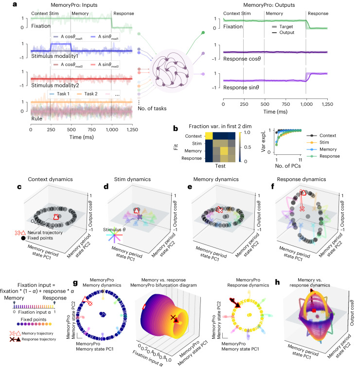
Fig. 1 Single-task network shared fixed points across task periods. a, Left: noisy fixation, stimulus (modality 1 and modality 2) and rule input time series (overlayed without noise for clarity). Noise was used during training, and analyses were performed on running the network without noise. Vertical lines divide task periods: context, stimulus, memory and response. Right: targets (thick lines) overlaid with outputs of a trained network (thin lines). Stim, stimulus task period. b, Fraction variance explained in each task period by top two PCs of neural state trajectories for 1,024 stimulus conditions from every other task period (left). We performed PCA on task period Y and then calculated how much variance it explained on task period X. Right: top 11 PCs of neural state trajectories for 1,024 stimulus conditions from each task period. c–f, State space plots for single-task network performing MemoryPro during context (c), stimulus (d), memory (e) and response (f) task periods. State trajectories and fixed points projected onto the first two PCs defined by state trajectories during the memory period on the x and y axes and the output weight vector (from Wout) associated with cosθstimulus on the z axis. We visualized fixed point locations for θstimulus = 0 (black dots) in all subpanels of Fig. 1 and additionally plotted state trajectories for other stimulus conditions (see 'Fixed points' in Methods for further details on fixed point identification). State trajectories (colored lines) are colored according to stimulus orientation with θstimulus = 0 highlighted in red, starting from ‘x’ and ending with ‘▴’. g, Interpolation between inputs for memory (α = 0) and response (α = 1) periods. Middle: fixed points for 20 intermediate α values (x axis) projected into top two memory period PCs (as in c–f) (y and z axes) with memory α = 0 (left) and response α = 1 (right) fixed points and trajectories. h, Fixed points for input interpolation between memory (blue) and response (yellow) inputs. State trajectories are colored according to stimulus orientation. Same axes as c–f. All subpanels were generated from the same network with hyperparameters: 256 units, softplus activation, diagonal initialization.
Fig. 1 Single-task network shared fixed points across task periods. a, Left: noisy fixation, stimulus (modality 1 and modality 2) and rule input time series (overlayed without noise for clarity). Noise was used during training, and analyses were performed on running the network without noise. Vertical lines divide task periods: context, stimulus, memory and response. Right: targets (thick lines) overlaid with outputs of a trained network (thin lines). Stim, stimulus task period. b, Fraction variance explained in each task period by top two PCs of neural state trajectories for 1,024 stimulus conditions from every other task period (left). We performed PCA on task period Y and then calculated how much variance it explained on task period X. Right: top 11 PCs of neural state trajectories for 1,024 stimulus conditions from each task period. c–f, State space plots for single-task network performing MemoryPro during context (c), stimulus (d), memory (e) and response (f) task periods. State trajectories and fixed points projected onto the first two PCs defined by state trajectories during the memory period on the x and y axes and the output weight vector (from Wout) associated with cosθstimulus on the z axis. We visualized fixed point locations for θstimulus = 0 (black dots) in all subpanels of Fig. 1 and additionally plotted state trajectories for other stimulus conditions (see 'Fixed points' in Methods for further details on fixed point identification). State trajectories (colored lines) are colored according to stimulus orientation with θstimulus = 0 highlighted in red, starting from ‘x’ and ending with ‘▴’. g, Interpolation between inputs for memory (α = 0) and response (α = 1) periods. Middle: fixed points for 20 intermediate α values (x axis) projected into top two memory period PCs (as in c–f) (y and z axes) with memory α = 0 (left) and response α = 1 (right) fixed points and trajectories. h, Fixed points for input interpolation between memory (blue) and response (yellow) inputs. State trajectories are colored according to stimulus orientation. Same axes as c–f. All subpanels were generated from the same network with hyperparameters: 256 units, softplus activation, diagonal initialization.CC BY · PubMed Central
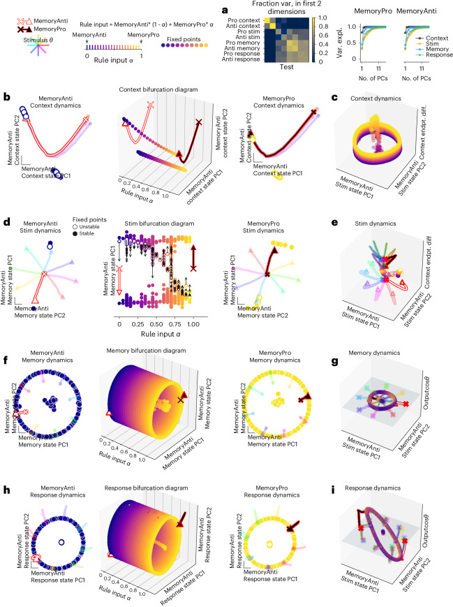
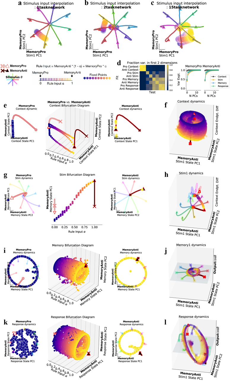
Fig. 2 Two-task networks shared fixed points across related tasks. a, Fraction variance explained in each task period by top two PCs of neural state trajectories for 1,024 stimulus conditions from every other task period (left). We performed PCA on task period Y and then calculated how much variance it explained on task period X. Right: top 10 PCs of neural state trajectories for 1,024 stimulus conditions from the same task period. b–i, Fixed points for interpolation between inputs for MemoryAnti (α = 0) and MemoryPro (α = 1) tasks during context (b,c), stimulus (d,e), memory (f,g) and response (h,i) periods. b, Middle, fixed points for 20 intermediate α values (x axis) projected into top two PCs defined by state trajectories during the context period of the MemoryAnti task (y and z axes) with MemoryAnti α = 0 (left) and MemoryPro α = 1 (right) fixed points and trajectories. c, Rule input interpolation between tasks, MemoryAnti (blue fixed points, white state trajectory) and MemoryPro (yellow fixed points, black state trajectory) projected into the top two MemoryAnti stimulus period state PCs and the vector connecting context period state endpoints on the z axis. d, Same as b for stimulus period, with unstable (open) and stable (closed) fixed points projected into top PC defined by the state trajectories during the memory period of the MemoryAnti task (y axis). Local linear dynamics around unstable fixed points are shown in black arrows: the state was initialized at the unstable fixed point and run forward for 10 steps. e, Same as c for stimulus period, projected into the top two MemoryAnti stimulus period state PCs and the vector connecting context period state endpoints on the z axis. f, Same as b for memory period, projected into top two PCs defined by the state trajectories during the memory period of the MemoryAnti task (y and z axes). g, Same as c for memory period, projected into the top two MemoryAnti stimulus period state PCs (x and y axes) and the output weight vector (from Wout) associated with cosθstimulus on the z axis. h, Same as b for response period, projected into top two PCs defined by the state trajectories during the response period of the MemoryAnti task (y and z axes). i, Same as g for response period. All subpanels were generated from the same network with hyperparameters: 256 units, softplus activation, diagonal initialization. endpt. diff., endpoint difference; Var. expl., variance explained.
Fig. 2 Two-task networks shared fixed points across related tasks. a, Fraction variance explained in each task period by top two PCs of neural state trajectories for 1,024 stimulus conditions from every other task period (left). We performed PCA on task period Y and then calculated how much variance it explained on task period X. Right: top 10 PCs of neural state trajectories for 1,024 stimulus conditions from the same task period. b–i, Fixed points for interpolation between inputs for MemoryAnti (α = 0) and MemoryPro (α = 1) tasks during context (b,c), stimulus (d,e), memory (f,g) and response (h,i) periods. b, Middle, fixed points for 20 intermediate α values (x axis) projected into top two PCs defined by state trajectories during the context period of the MemoryAnti task (y and z axes) with MemoryAnti α = 0 (left) and MemoryPro α = 1 (right) fixed points and trajectories. c, Rule input interpolation between tasks, MemoryAnti (blue fixed points, white state trajectory) and MemoryPro (yellow fixed points, black state trajectory) projected into the top two MemoryAnti stimulus period state PCs and the vector connecting context period state endpoints on the z axis. d, Same as b for stimulus period, with unstable (open) and stable (closed) fixed points projected into top PC defined by the state trajectories during the memory period of the MemoryAnti task (y axis). Local linear dynamics around unstable fixed points are shown in black arrows: the state was initialized at the unstable fixed point and run forward for 10 steps. e, Same as c for stimulus period, projected into the top two MemoryAnti stimulus period state PCs and the vector connecting context period state endpoints on the z axis. f, Same as b for memory period, projected into top two PCs defined by the state trajectories during the memory period of the MemoryAnti task (y and z axes). g, Same as c for memory period, projected into the top two MemoryAnti stimulus period state PCs (x and y axes) and the output weight vector (from Wout) associated with cosθstimulus on the z axis. h, Same as b for response period, projected into top two PCs defined by the state trajectories during the response period of the MemoryAnti task (y and z axes). i, Same as g for response period. All subpanels were generated from the same network with hyperparameters: 256 units, softplus activation, diagonal initialization. endpt. diff., endpoint difference; Var. expl., variance explained.CC BY · PubMed Central
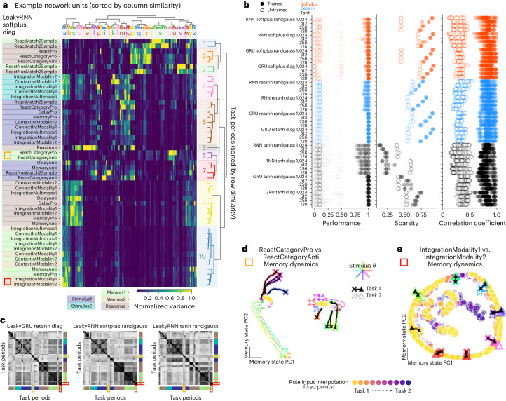
Fig. 3 Modular organization in 15 task networks was not dependent on activation function, network initialization or size. a, Variance matrix: variance of unit activations across stimulus conditions, normalized across task periods (columns normalized by the maximum entry in each column). Rows and columns were sorted according to similarity ('Clusters' in Methods). Colors along the left side label each task period type (dark blue: initial stimulus; light blue: second stimulus; light green: initial memory; yellow: second memory; brown: response). Notice that blocks with high variance belong to same task period types (similar colors). a,c–e, Orange and red rectangles highlight category memory (ReactCategoryPro, ReactCategoryAnti) and continuous memory (IntegrationModality1, IntegrationModality2) tasks, respectively. b, Left: performance across all tasks for three networks of each of 48 hyperparameter settings. Middle: sparsity of the task variance measured as the fraction of entries <15% maximum unit variance. Right: task period correlation matrix (examples shown in c) for trained and untrained networks are sorted according to rows in a and correlated to trained networks for all other hyperparameter settings. c, Correlation matrix of rows in variance matrix (as in a) for three different example networks; rows and columns sorted according to rows in a. Colors along the bottom and right axes label each task period type (dark blue: initial stimulus; light blue: second stimulus; light green: initial memory; yellow: second memory; brown: response). Notice that blocks with high correlation belong to the same task period types (similar colors). d, Shared point attractors for two category memory tasks as seen by input interpolation across tasks during memory period. State trajectories for eight stimulus conditions (colored by stimulus direction) starting from ‘x’ projected in PC space, defined by concatenating memory period state trajectories from both tasks for ReactCategoryPro (black) and ReactCategoryAnti (white) tasks. Rule input interpolation across tasks during memory period with fixed points for intermediate rule input conditions in filled circles. e, Same as d for two continuous circular variable memory tasks, highlighting shared ring attractors. State trajectories starting from ‘x’ projected in PC space, defined by concatenating memory period state trajectories from both tasks for IntegrationModality1 (black) and IntegrationModality2 (white) tasks. Panels a, d and e were generated from the same network with hyperparameters: 128 units, softplus activation, diagonal initialization. randgauss, random Gaussian.
Fig. 3 Modular organization in 15 task networks was not dependent on activation function, network initialization or size. a, Variance matrix: variance of unit activations across stimulus conditions, normalized across task periods (columns normalized by the maximum entry in each column). Rows and columns were sorted according to similarity ('Clusters' in Methods). Colors along the left side label each task period type (dark blue: initial stimulus; light blue: second stimulus; light green: initial memory; yellow: second memory; brown: response). Notice that blocks with high variance belong to same task period types (similar colors). a,c–e, Orange and red rectangles highlight category memory (ReactCategoryPro, ReactCategoryAnti) and continuous memory (IntegrationModality1, IntegrationModality2) tasks, respectively. b, Left: performance across all tasks for three networks of each of 48 hyperparameter settings. Middle: sparsity of the task variance measured as the fraction of entries <15% maximum unit variance. Right: task period correlation matrix (examples shown in c) for trained and untrained networks are sorted according to rows in a and correlated to trained networks for all other hyperparameter settings. c, Correlation matrix of rows in variance matrix (as in a) for three different example networks; rows and columns sorted according to rows in a. Colors along the bottom and right axes label each task period type (dark blue: initial stimulus; light blue: second stimulus; light green: initial memory; yellow: second memory; brown: response). Notice that blocks with high correlation belong to the same task period types (similar colors). d, Shared point attractors for two category memory tasks as seen by input interpolation across tasks during memory period. State trajectories for eight stimulus conditions (colored by stimulus direction) starting from ‘x’ projected in PC space, defined by concatenating memory period state trajectories from both tasks for ReactCategoryPro (black) and ReactCategoryAnti (white) tasks. Rule input interpolation across tasks during memory period with fixed points for intermediate rule input conditions in filled circles. e, Same as d for two continuous circular variable memory tasks, highlighting shared ring attractors. State trajectories starting from ‘x’ projected in PC space, defined by concatenating memory period state trajectories from both tasks for IntegrationModality1 (black) and IntegrationModality2 (white) tasks. Panels a, d and e were generated from the same network with hyperparameters: 128 units, softplus activation, diagonal initialization. randgauss, random Gaussian.CC BY · PubMed Central
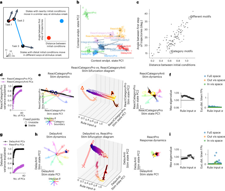
Fig. 4 Tasks with similar stimulus computations were in nearby parts of state space and shared dynamical motifs. a, Schematic of analyses in b and c. b, The state for each trial (colored dot for each of 20 trials on each task) at the end of the context period (just before stimulus period) projected onto the top two PCs defined by the state at the end of the context period for all tasks. Trial–trial variation is due to input noise, independent noise and random initial conditions. Trials colored by similar stimulus computations as given by task definitions: pro delayed (light blue), anti delayed (red), pro integration (steel blue), categorization (pink), pro reaction (green) and anti reaction (orange). See Supplementary Table 1 for motif definitions. c, Euclidean distance between pairs of trials from different tasks at the end of the context period plotted against cosine angle between same pair after stimulus onset for a particular stimulus input, θstimulus, for one timestep and then averaged across stimulus angle inputs. Pairs of tasks in d–i are circled and labeled: ‘Category Motif’: ReactCategoryPro and ReactCategoryAnti (d–f) and ‘Different Motifs’: DelayAnti and ReactPro (g–i). d, Fraction of variance explained for ReactCategoryPro task by the ReactCategoryAnti task PCs (purple) compared to its own PCs (black) for five trained networks with different random seeds. e, Rule input interpolation across category tasks for one stimulus angle. Middle, unstable (open) and stable (closed) fixed points for 20 intermediate α values (x axis) projected onto top two PCs defined by state trajectories during the stimulus period of the ReactCategoryPro task (y and z axes) with ReactCategoryPro α = 0 (left) and ReactCategoryAnti α = 1 (right) fixed points and trajectories for eight different stimulus angles (rainbow colors). Expanding dimensions around unstable fixed points are visualized as black lines. f, Left, maximum real eigenvalue for the linearization of the state update around each fixed point for the single unstable fixed point closest to the state at the end of the stimulus period for 20 consecutive α values between 0 and 1. Right, Euclidean distance between consecutive fixed points in the full state space (blue), outside of the visualized subspace in e (orange) and within the visualized space (green). We analyzed only one unstable fixed point that is most proximal to the end of the state trajectory for each input condition to highlight the task relevant fixed point ('Analysis of fixed points for interpolated inputs' in Methods). g–i, ‘Different Motifs’: DelayAnti and ReactPro. Same as d–f but for DelayAnti and ReactPro tasks. Note that a response is required at stimulus onset for the ReactPro task; therefore, the stimulus period is the same as the response period. i, Left, maximum real eigenvalue for the linearization of the state update around each fixed point for the single fixed point closest to the state at the end of the stimulus period for 20 consecutive α values between 0 and 1. Right, Euclidean distance between consecutive fixed points in the full state space (blue), outside of the visualized subspace in h (orange) and within the visualized space (green). We analyzed one fixed point that is most proximal to the end of the state trajectory for each input condition. Panels b, c, e, f, h and i were generated from the same network as in Fig. 3a with hyperparameters: LeakyRNN, 128 units, softplus activation, diagonal initialization. Other networks in d and g use the same hyperparameters. deg, degrees; endpt., endpoint; Euc.dist. btwn, Euclidian distance between; FP, fixed point; vis, visualized.
Fig. 4 Tasks with similar stimulus computations were in nearby parts of state space and shared dynamical motifs. a, Schematic of analyses in b and c. b, The state for each trial (colored dot for each of 20 trials on each task) at the end of the context period (just before stimulus period) projected onto the top two PCs defined by the state at the end of the context period for all tasks. Trial–trial variation is due to input noise, independent noise and random initial conditions. Trials colored by similar stimulus computations as given by task definitions: pro delayed (light blue), anti delayed (red), pro integration (steel blue), categorization (pink), pro reaction (green) and anti reaction (orange). See Supplementary Table 1 for motif definitions. c, Euclidean distance between pairs of trials from different tasks at the end of the context period plotted against cosine angle between same pair after stimulus onset for a particular stimulus input, θstimulus, for one timestep and then averaged across stimulus angle inputs. Pairs of tasks in d–i are circled and labeled: ‘Category Motif’: ReactCategoryPro and ReactCategoryAnti (d–f) and ‘Different Motifs’: DelayAnti and ReactPro (g–i). d, Fraction of variance explained for ReactCategoryPro task by the ReactCategoryAnti task PCs (purple) compared to its own PCs (black) for five trained networks with different random seeds. e, Rule input interpolation across category tasks for one stimulus angle. Middle, unstable (open) and stable (closed) fixed points for 20 intermediate α values (x axis) projected onto top two PCs defined by state trajectories during the stimulus period of the ReactCategoryPro task (y and z axes) with ReactCategoryPro α = 0 (left) and ReactCategoryAnti α = 1 (right) fixed points and trajectories for eight different stimulus angles (rainbow colors). Expanding dimensions around unstable fixed points are visualized as black lines. f, Left, maximum real eigenvalue for the linearization of the state update around each fixed point for the single unstable fixed point closest to the state at the end of the stimulus period for 20 consecutive α values between 0 and 1. Right, Euclidean distance between consecutive fixed points in the full state space (blue), outside of the visualized subspace in e (orange) and within the visualized space (green). We analyzed only one unstable fixed point that is most proximal to the end of the state trajectory for each input condition to highlight the task relevant fixed point ('Analysis of fixed points for interpolated inputs' in Methods). g–i, ‘Different Motifs’: DelayAnti and ReactPro. Same as d–f but for DelayAnti and ReactPro tasks. Note that a response is required at stimulus onset for the ReactPro task; therefore, the stimulus period is the same as the response period. i, Left, maximum real eigenvalue for the linearization of the state update around each fixed point for the single fixed point closest to the state at the end of the stimulus period for 20 consecutive α values between 0 and 1. Right, Euclidean distance between consecutive fixed points in the full state space (blue), outside of the visualized subspace in h (orange) and within the visualized space (green). We analyzed one fixed point that is most proximal to the end of the state trajectory for each input condition. Panels b, c, e, f, h and i were generated from the same network as in Fig. 3a with hyperparameters: LeakyRNN, 128 units, softplus activation, diagonal initialization. Other networks in d and g use the same hyperparameters. deg, degrees; endpt., endpoint; Euc.dist. btwn, Euclidian distance between; FP, fixed point; vis, visualized.CC BY · PubMed Central
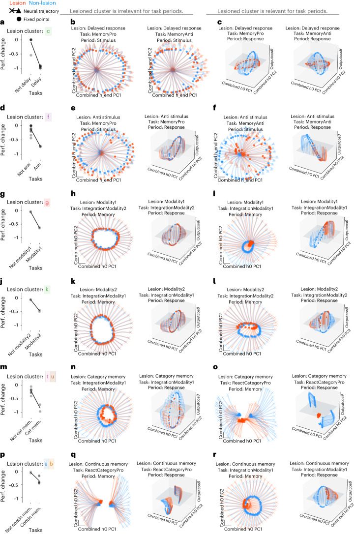
Fig. 5 Unit cluster lesions had modular effects on task period clusters that shared the same dynamical motif. a–c, Delayed response lesion. a, Fraction performance change (each point is one task) after delayed response (cluster c in Fig. 3a) lesion by setting unit output to zero for units within cluster with high variance during the response period of delayed response tasks (see Supplementary Table 1 for motif definitions). b, Fixed points (filled circles) and state trajectories (starting from ‘x’ and ending with ‘▴’) during the performance of MemoryPro and MemoryAnti stimulus periods in lesioned (orange) and full (blue) network projected into the first two PCs (x and y axes) defined by the full and lesioned network state at the last timestep of the stimulus period. Stimulus period dynamics should not be relevant for the delayed response unit cluster lesion. As a result, fixed points and state trajectories diverge minimally from the full network. c, Same as b during the response periods in lesioned (orange) and full (blue) network projected into the first two PCs (x and y axes) defined by the full and lesioned network state at the first timestep of the response period and the output weight vector (from Wout) associated with cosθstimulus on the z axis. Response period dynamics should be relevant for the delayed response unit cluster lesion. As a result, lesion prevents fixed points from rotating into output potent space and has a marked impact on network performance. d–f, Anti stimulus lesion. d, Same as a for anti stimulus (cluster f in Fig. 3a) during irrelevant MemoryPro stimulus and response task periods (e) and relevant MemoryAnti stimulus and response task periods (f). Fixed points and activity are projected onto the first two PCs defined by the network state at the last timestep of the stimulus period for both the lesioned and full network (x and y axes) (left) and the first timestep of the response period and the output weight vector (from Wout) associated with cosθstimulus on the z axis (right). g–i, Modality 1 Lesion. g, Same as a for Modality 1 (cluster g in Fig. 3a). h, Irrelevant IntegrationModality2 stimulus and response task periods. i, Relevant IntegrationModality1 stimulus and response task periods. Fixed points and activity are projected onto the first two PCs (x and y axes) defined by the network state at the first timestep of the memory task period for both the lesioned and full network and the output weight vector (from Wout) associated with cosθstimulus on the z axis. j–l, Modality 2 Lesion. j, Same as a for Modality 2 (cluster k in Fig. 3a). k, Irrelevant IntegrationModality1 stimulus and response task periods. l, Relevant IntegrationModality2 stimulus and response task periods. Fixed points and activity are projected onto the first two PCs (x and y axes) defined by the network state at the first timestep of the memory task period for both the lesioned and full network (left) and the first timestep of the response task period for both the lesioned and full network and the output weight vector (from Wout) associated with cosθstimulus on the z axis (right). m–o, Category memory lesion. m, Same as a for category memory (clusters t and u in Fig. 3a). n, Irrelevant IntegrationModality1 memory and response task periods. o, Relevant ReactCategoryPro memory and response task periods. Fixed points and activity are projected onto the first two PCs (x and y axes) defined by the network state at the first timestep of the memory task period for both the lesioned and full network (left) and the first timestep of the response task period for both the lesioned and full network and the output weight vector (from Wout) associated with cosθstimulus on the z axis (right). p–r, Continuous memory lesion. p, Same as a for continuous memory (clusters a and b in Fig. 3a). q, Irrelevant ReactCategoryPro memory and response task periods. r, Relevant IntegrationModality1 memory and response task periods. Fixed points and activity are projected onto the first two PCs (x and y axes) defined by the network state at the first timestep of the memory task period for both the lesioned and full network and the output weight vector (from Wout) associated with cosθstimulus on the z axis. All panels were generated from the same network as in Fig. 3a with hyperparameters: LeakyRNN, 128 units, softplus activation, diagonal initialization. Perf., performance. h0 is the state at the beginning of the task period and h_end is the state at the end of the task period.
Fig. 5 Unit cluster lesions had modular effects on task period clusters that shared the same dynamical motif. a–c, Delayed response lesion. a, Fraction performance change (each point is one task) after delayed response (cluster c in Fig. 3a) lesion by setting unit output to zero for units within cluster with high variance during the response period of delayed response tasks (see Supplementary Table 1 for motif definitions). b, Fixed points (filled circles) and state trajectories (starting from ‘x’ and ending with ‘▴’) during the performance of MemoryPro and MemoryAnti stimulus periods in lesioned (orange) and full (blue) network projected into the first two PCs (x and y axes) defined by the full and lesioned network state at the last timestep of the stimulus period. Stimulus period dynamics should not be relevant for the delayed response unit cluster lesion. As a result, fixed points and state trajectories diverge minimally from the full network. c, Same as b during the response periods in lesioned (orange) and full (blue) network projected into the first two PCs (x and y axes) defined by the full and lesioned network state at the first timestep of the response period and the output weight vector (from Wout) associated with cosθstimulus on the z axis. Response period dynamics should be relevant for the delayed response unit cluster lesion. As a result, lesion prevents fixed points from rotating into output potent space and has a marked impact on network performance. d–f, Anti stimulus lesion. d, Same as a for anti stimulus (cluster f in Fig. 3a) during irrelevant MemoryPro stimulus and response task periods (e) and relevant MemoryAnti stimulus and response task periods (f). Fixed points and activity are projected onto the first two PCs defined by the network state at the last timestep of the stimulus period for both the lesioned and full network (x and y axes) (left) and the first timestep of the response period and the output weight vector (from Wout) associated with cosθstimulus on the z axis (right). g–i, Modality 1 Lesion. g, Same as a for Modality 1 (cluster g in Fig. 3a). h, Irrelevant IntegrationModality2 stimulus and response task periods. i, Relevant IntegrationModality1 stimulus and response task periods. Fixed points and activity are projected onto the first two PCs (x and y axes) defined by the network state at the first timestep of the memory task period for both the lesioned and full network and the output weight vector (from Wout) associated with cosθstimulus on the z axis. j–l, Modality 2 Lesion. j, Same as a for Modality 2 (cluster k in Fig. 3a). k, Irrelevant IntegrationModality1 stimulus and response task periods. l, Relevant IntegrationModality2 stimulus and response task periods. Fixed points and activity are projected onto the first two PCs (x and y axes) defined by the network state at the first timestep of the memory task period for both the lesioned and full network (left) and the first timestep of the response task period for both the lesioned and full network and the output weight vector (from Wout) associated with cosθstimulus on the z axis (right). m–o, Category memory lesion. m, Same as a for category memory (clusters t and u in Fig. 3a). n, Irrelevant IntegrationModality1 memory and response task periods. o, Relevant ReactCategoryPro memory and response task periods. Fixed points and activity are projected onto the first two PCs (x and y axes) defined by the network state at the first timestep of the memory task period for both the lesioned and full network (left) and the first timestep of the response task period for both the lesioned and full network and the output weight vector (from Wout) associated with cosθstimulus on the z axis (right). p–r, Continuous memory lesion. p, Same as a for continuous memory (clusters a and b in Fig. 3a). q, Irrelevant ReactCategoryPro memory and response task periods. r, Relevant IntegrationModality1 memory and response task periods. Fixed points and activity are projected onto the first two PCs (x and y axes) defined by the network state at the first timestep of the memory task period for both the lesioned and full network and the output weight vector (from Wout) associated with cosθstimulus on the z axis. All panels were generated from the same network as in Fig. 3a with hyperparameters: LeakyRNN, 128 units, softplus activation, diagonal initialization. Perf., performance. h0 is the state at the beginning of the task period and h_end is the state at the end of the task period.CC BY · PubMed Central
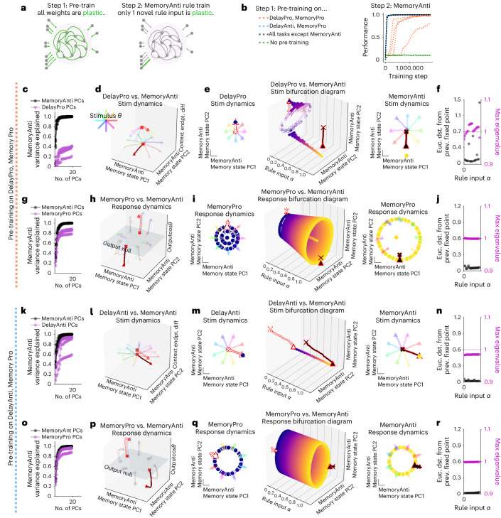
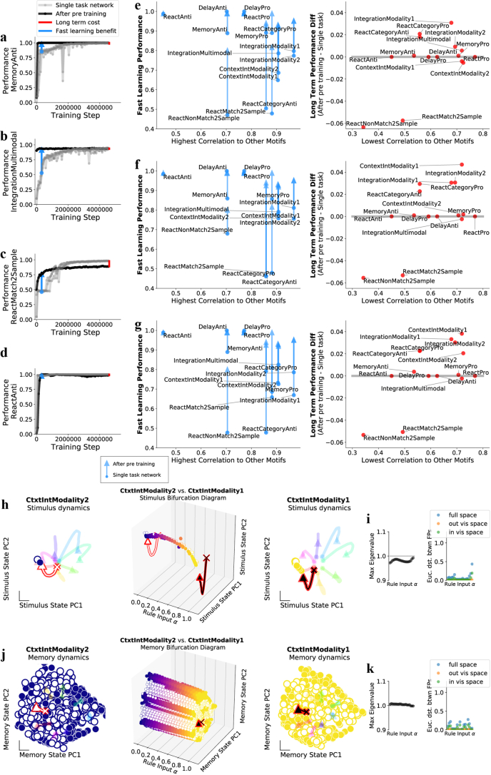
Fig. 6 Dynamical motifs were reused for fast learning of novel tasks with familiar computational elements. a, Schematic of two-stage learning. Networks were pre-trained on a set of tasks while all weights were plastic. The same network was then trained on a novel task by only learning weights for a single new one-hot rule input. b, Left; networks were pre-trained on two tasks that include pro stimulus and continuous memory motifs (orange), anti stimulus and continuous memory motifs (blue), all motifs (black) and no motifs (green). See Supplementary Table 1 for motif definitions. Right: performance during MemoryAnti task rule input weight training after pre-training on various sets of motifs for five different networks each. c–j, Network pre-trained on DelayPro and MemoryPro tasks (pro stimulus and continuous memory motifs) was then trained to perform MemoryAnti through weight changes to the MemoryAnti rule input (Nrec × 1 vector). c, Fraction of MemoryAnti stimulus period variance explained by MemoryAnti stimulus period PCs (black) and DelayPro stimulus period PCs (purple) quantifies the extent to which both pro and anti tasks are in a similar subspace during the stimulus period. d, Stimulus period activity for DelayPro (white) and MemoryAnti (black) tasks for eight different stimulus angles (rainbow colors) projected into PC space (x and y axes) defined by state trajectories during MemoryAnti task and context period state endpoint difference between both tasks (z axis). e, Rule input interpolation across tasks for one stimulus angle. Middle: unstable (open) and stable (closed) fixed points for 20 intermediate α values (x axis) projected onto top two PCs defined by state trajectories during the memory period of the MemoryAnti task (y and z axes) with DelayPro α = 0 (left) and MemoryAnti α = 1 (right) fixed points and activity for eight different stimulus angles (rainbow colors). f, Euclidean distance between fixed points (black) and maximum real eigenvalue for the linearization of the state update around each fixed point (purple) for the single fixed point closest to the state at the end of the stimulus period for 20 consecutive α values between 0 and 1. Analyzing only one fixed point that is most proximal to the end of the state trajectory for each input condition ('Analysis of fixed points for interpolated inputs' in Methods). g–j, Same as c–f for response period of MemoryPro and MemoryAnti tasks. k–r, Network pre-trained on DelayAnti and MemoryPro tasks (anti stimulus and continuous memory motifs) was then trained to perform MemoryAnti task through weight changes to the MemoryAnti rule input (length Nrec vector). k–n, Same as c–f for stimulus period of DelayAnti and MemoryAnti tasks with pre-training on DelayAnti and MemoryPro tasks. o–r, Same as c–f for response period of MemoryPro and MemoryAnti tasks with pre-training on DelayAnti and MemoryPro tasks. d–f and h–j were generated from one network, and l–n and p–r were generated from a different network, both with hyperparameters: LeakyRNN, 256 units, softplus activation, diagonal initialization. Euc. dst., Euclidian distance.
Fig. 6 Dynamical motifs were reused for fast learning of novel tasks with familiar computational elements. a, Schematic of two-stage learning. Networks were pre-trained on a set of tasks while all weights were plastic. The same network was then trained on a novel task by only learning weights for a single new one-hot rule input. b, Left; networks were pre-trained on two tasks that include pro stimulus and continuous memory motifs (orange), anti stimulus and continuous memory motifs (blue), all motifs (black) and no motifs (green). See Supplementary Table 1 for motif definitions. Right: performance during MemoryAnti task rule input weight training after pre-training on various sets of motifs for five different networks each. c–j, Network pre-trained on DelayPro and MemoryPro tasks (pro stimulus and continuous memory motifs) was then trained to perform MemoryAnti through weight changes to the MemoryAnti rule input (Nrec × 1 vector). c, Fraction of MemoryAnti stimulus period variance explained by MemoryAnti stimulus period PCs (black) and DelayPro stimulus period PCs (purple) quantifies the extent to which both pro and anti tasks are in a similar subspace during the stimulus period. d, Stimulus period activity for DelayPro (white) and MemoryAnti (black) tasks for eight different stimulus angles (rainbow colors) projected into PC space (x and y axes) defined by state trajectories during MemoryAnti task and context period state endpoint difference between both tasks (z axis). e, Rule input interpolation across tasks for one stimulus angle. Middle: unstable (open) and stable (closed) fixed points for 20 intermediate α values (x axis) projected onto top two PCs defined by state trajectories during the memory period of the MemoryAnti task (y and z axes) with DelayPro α = 0 (left) and MemoryAnti α = 1 (right) fixed points and activity for eight different stimulus angles (rainbow colors). f, Euclidean distance between fixed points (black) and maximum real eigenvalue for the linearization of the state update around each fixed point (purple) for the single fixed point closest to the state at the end of the stimulus period for 20 consecutive α values between 0 and 1. Analyzing only one fixed point that is most proximal to the end of the state trajectory for each input condition ('Analysis of fixed points for interpolated inputs' in Methods). g–j, Same as c–f for response period of MemoryPro and MemoryAnti tasks. k–r, Network pre-trained on DelayAnti and MemoryPro tasks (anti stimulus and continuous memory motifs) was then trained to perform MemoryAnti task through weight changes to the MemoryAnti rule input (length Nrec vector). k–n, Same as c–f for stimulus period of DelayAnti and MemoryAnti tasks with pre-training on DelayAnti and MemoryPro tasks. o–r, Same as c–f for response period of MemoryPro and MemoryAnti tasks with pre-training on DelayAnti and MemoryPro tasks. d–f and h–j were generated from one network, and l–n and p–r were generated from a different network, both with hyperparameters: LeakyRNN, 256 units, softplus activation, diagonal initialization. Euc. dst., Euclidian distance.CC BY · PubMed Central
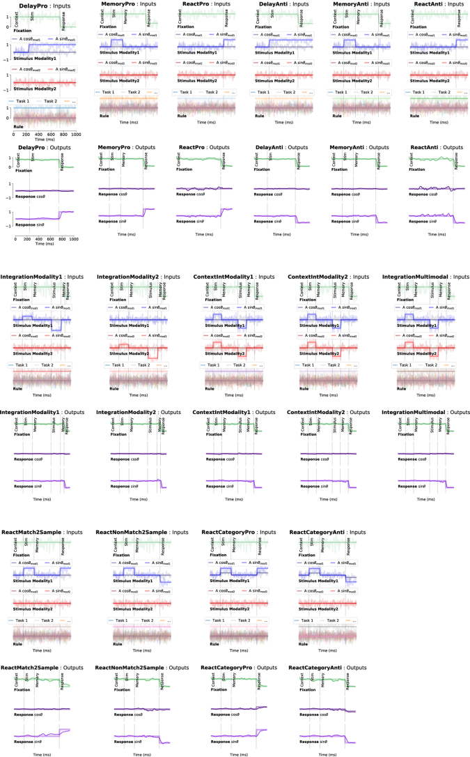
Extended Data Fig. 1 Inputs and outputs for each task for one example trial. One panel for each task. Top: Noisy fixation, stimulus (modality 1 and 2), and rule input time-series (overlayed without noise for clarity). Noise was used during training while analyses were performed by running the network without noise (except Fig. 4b, which was run with noise). Vertical lines divide task periods. Bottom: Targets (thick lines) overlaid with outputs of a trained network (thin lines).
Extended Data Fig. 1 Inputs and outputs for each task for one example trial. One panel for each task. Top: Noisy fixation, stimulus (modality 1 and 2), and rule input time-series (overlayed without noise for clarity). Noise was used during training while analyses were performed by running the network without noise (except Fig. 4b, which was run with noise). Vertical lines divide task periods. Bottom: Targets (thick lines) overlaid with outputs of a trained network (thin lines).CC BY · PubMed Central
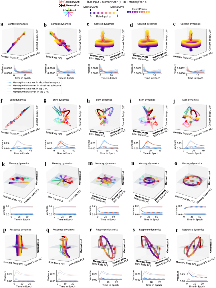
Extended Data Fig. 2 Additional visualizations of shared fixed points across MemoryPro and MemoryAnti tasks in a two-task network. These figures are meant to provide more intuition for high dimensional dynamics by presenting fixed point interpolations and state trajectories in more dimensions (top) with a quantification of variance of the network state across stimulus conditions plotted through time in each subspace (bottom). Fixed points and state trajectories for interpolation between rule inputs for MemoryAnti (α = 0) and MemoryPro (α = 1) tasks during (a-e) context (f-j) stimulus (k-o) memory (p-t) and response periods. (a-e) top: Context period fixed points for rule input-interpolation between tasks, MemoryAnti (blue fixed points, white state trajectory) and MemoryPro (yellow fixed points, black state trajectory) projected into the top two principal components (PCs) identified by performing PCA on concatenated state trajectories from MemoryPro and MemoryAnti (a) context task periods (b) stimulus task periods (c) MemoryPro stimulus task period only (d) MemoryAnti stimulus task period only (e) memory task periods. (a-e) bottom: Variance of state trajectories across stimulus conditions plotted through time during MemoryPro (blue, dotted) and MemoryAnti (orange, dotted) projected in the associated (above) visualized subspace. Solids lines indicate variance of state trajectories during the context period, projected into their own top two PC subspace. This provides a reference for how much variance the visualization captures relative to the PC subspace for each task period. Note, there is little variance during the context period, especially in networks only trained to perform a small number of tasks. Therefore, visualizations in the leftmost column and top row do not provide much insight about the dynamics, but more clearly show the relationship between the stable fixed point that guides the state during the context period and the ring attractor during the memory period, both shared across tasks. Remember, inputs during context and memory periods are identical; and therefore, fixed points are identical across these task periods. (f-j) Same as a-e for stimulus period fixed points and state trajectories. These panels show that the (g) initial stimulus response is in an overlapping subspace; however, (h,i) there are mostly nonoverlapping subspaces that capture maximal stimulus variance across both tasks. (j) By the end of the stimulus period, the state moves into an aligned memory subspace across both tasks. (k-o) Same as a-e for memory period fixed points and activity. (l) Early stimulus period representation is mostly orthogonal to memory period representation. (m-n) State trajectories move out of separate stimulus subspaces early in the memory period. (o) Little movement of state trajectories in shared memory subspace throughout memory period. (p-t) Same as a-e for response period fixed points and state trajectories show (r-t) similar organization of fixed point and trajectories in all subspaces. All subpanels generated from the same network as in Fig. 2 with hyperparameters: 256 units, softplus activation, diagonal initialization.
Extended Data Fig. 2 Additional visualizations of shared fixed points across MemoryPro and MemoryAnti tasks in a two-task network. These figures are meant to provide more intuition for high dimensional dynamics by presenting fixed point interpolations and state trajectories in more dimensions (top) with a quantification of variance of the network state across stimulus conditions plotted through time in each subspace (bottom). Fixed points and state trajectories for interpolation between rule inputs for MemoryAnti (α = 0) and MemoryPro (α = 1) tasks during (a-e) context (f-j) stimulus (k-o) memory (p-t) and response periods. (a-e) top: Context period fixed points for rule input-interpolation between tasks, MemoryAnti (blue fixed points, white state trajectory) and MemoryPro (yellow fixed points, black state trajectory) projected into the top two principal components (PCs) identified by performing PCA on concatenated state trajectories from MemoryPro and MemoryAnti (a) context task periods (b) stimulus task periods (c) MemoryPro stimulus task period only (d) MemoryAnti stimulus task period only (e) memory task periods. (a-e) bottom: Variance of state trajectories across stimulus conditions plotted through time during MemoryPro (blue, dotted) and MemoryAnti (orange, dotted) projected in the associated (above) visualized subspace. Solids lines indicate variance of state trajectories during the context period, projected into their own top two PC subspace. This provides a reference for how much variance the visualization captures relative to the PC subspace for each task period. Note, there is little variance during the context period, especially in networks only trained to perform a small number of tasks. Therefore, visualizations in the leftmost column and top row do not provide much insight about the dynamics, but more clearly show the relationship between the stable fixed point that guides the state during the context period and the ring attractor during the memory period, both shared across tasks. Remember, inputs during context and memory periods are identical; and therefore, fixed points are identical across these task periods. (f-j) Same as a-e for stimulus period fixed points and state trajectories. These panels show that the (g) initial stimulus response is in an overlapping subspace; however, (h,i) there are mostly nonoverlapping subspaces that capture maximal stimulus variance across both tasks. (j) By the end of the stimulus period, the state moves into an aligned memory subspace across both tasks. (k-o) Same as a-e for memory period fixed points and activity. (l) Early stimulus period representation is mostly orthogonal to memory period representation. (m-n) State trajectories move out of separate stimulus subspaces early in the memory period. (o) Little movement of state trajectories in shared memory subspace throughout memory period. (p-t) Same as a-e for response period fixed points and state trajectories show (r-t) similar organization of fixed point and trajectories in all subspaces. All subpanels generated from the same network as in Fig. 2 with hyperparameters: 256 units, softplus activation, diagonal initialization.CC BY · PubMed Central
Extended Data Fig. 3 Fixed point structure is dependent on other tasks the network is trained to perform and fixed points are shared regardless of network size or noise. (a-c) Networks were trained to perform 1, 2 or 15 tasks with the same hyperparameters: LeakyRNN, 256 units, softplus activation, diagonal initialization. (a) One-task network fixed points for interpolated inputs across stimulus conditions 0°(blue)→45° (yellow), reveals one fixed point that moves dependent on stimulus input conditions. Trajectories colored according to stimulus orientation. Additional fixed points are revealed in (b) two task network and (c) 15 task network. Subpanels a-c reveal that training a network on multiple tasks results in additional fixed points that persist across different contextual inputs. This highlights a key point, that neural dynamics in real brains will likely be a product of all the tasks animals perform. This result could guide future perturbation experiments and the study of error trials. Rotations of fixed points in the PC spaces of different networks is irrelevant to this point. (d-l) Large networks with no noise also share fixed points. Example two task network trained to perform MemoryPro and MemoryAnti tasks with hyperparameters: LeakyRNN, 1024 units, softplus activation, diagonal initialization and no input noise or independent noise (see equations 5 and 10 in Methods for noise definitions). (d) Fraction variance explained in each task period by left: top two principal components (PCs) of state trajectories for 1024 stimulus conditions from every other task period. We performed PCA on task period Y then calculated how much variance it explained on task period X. right: top ten PCs of state trajectories for 1024 stimulus conditions from the each task period. (e-l) Fixed points for interpolation between inputs for MemoryPro (α = 0) and MemoryAnti (α = 1) tasks during (e,f) context (g,h) stimulus (i,j) memory (k,l) and response periods. (e) middle: Fixed points for 20 intermediate α values (x-axis) projected into top two PCs defined by state trajectories during the context period of the MemoryAnti task (y and z-axis) with (left) MemoryPro α = 0 and (right) MemoryAnti α = 1 fixed points and trajectories. (f) Fixed points for rule input-interpolation between tasks, MemoryPro (blue fixed points, white state trajectory) and MemoryAnti (yellow fixed points, black state trajectory) projected into the top two MemoryAnti stimulus period state PCs and the dimension separating both tasks at the end of the context period (z axis). (g) Same as e for stimulus period, projected into top PC defined by state trajectories during the memory period of the MemoryAnti task (y-axis) (h) Same as f for stimulus period. (i) Same as e for memory period, projected into top two PCs defined by state trajectories during the memory period of the MemoryAnti task (y and z-axes). (j) Same as h for memory period, projected into the top two MemoryAnti stimulus period state PCs (x and y-axes) and the output weight vector (from Wout) associated with cosθstimulus on the z-axis. (k) Same as e for response period, projected into top two PCs defined by the state trajectories during the response period of the MemoryAnti task (y and z-axes). (l) Same as j for response period.
Extended Data Fig. 3 Fixed point structure is dependent on other tasks the network is trained to perform and fixed points are shared regardless of network size or noise. (a-c) Networks were trained to perform 1, 2 or 15 tasks with the same hyperparameters: LeakyRNN, 256 units, softplus activation, diagonal initialization. (a) One-task network fixed points for interpolated inputs across stimulus conditions 0°(blue)→45° (yellow), reveals one fixed point that moves dependent on stimulus input conditions. Trajectories colored according to stimulus orientation. Additional fixed points are revealed in (b) two task network and (c) 15 task network. Subpanels a-c reveal that training a network on multiple tasks results in additional fixed points that persist across different contextual inputs. This highlights a key point, that neural dynamics in real brains will likely be a product of all the tasks animals perform. This result could guide future perturbation experiments and the study of error trials. Rotations of fixed points in the PC spaces of different networks is irrelevant to this point. (d-l) Large networks with no noise also share fixed points. Example two task network trained to perform MemoryPro and MemoryAnti tasks with hyperparameters: LeakyRNN, 1024 units, softplus activation, diagonal initialization and no input noise or independent noise (see equations 5 and 10 in Methods for noise definitions). (d) Fraction variance explained in each task period by left: top two principal components (PCs) of state trajectories for 1024 stimulus conditions from every other task period. We performed PCA on task period Y then calculated how much variance it explained on task period X. right: top ten PCs of state trajectories for 1024 stimulus conditions from the each task period. (e-l) Fixed points for interpolation between inputs for MemoryPro (α = 0) and MemoryAnti (α = 1) tasks during (e,f) context (g,h) stimulus (i,j) memory (k,l) and response periods. (e) middle: Fixed points for 20 intermediate α values (x-axis) projected into top two PCs defined by state trajectories during the context period of the MemoryAnti task (y and z-axis) with (left) MemoryPro α = 0 and (right) MemoryAnti α = 1 fixed points and trajectories. (f) Fixed points for rule input-interpolation between tasks, MemoryPro (blue fixed points, white state trajectory) and MemoryAnti (yellow fixed points, black state trajectory) projected into the top two MemoryAnti stimulus period state PCs and the dimension separating both tasks at the end of the context period (z axis). (g) Same as e for stimulus period, projected into top PC defined by state trajectories during the memory period of the MemoryAnti task (y-axis) (h) Same as f for stimulus period. (i) Same as e for memory period, projected into top two PCs defined by state trajectories during the memory period of the MemoryAnti task (y and z-axes). (j) Same as h for memory period, projected into the top two MemoryAnti stimulus period state PCs (x and y-axes) and the output weight vector (from Wout) associated with cosθstimulus on the z-axis. (k) Same as e for response period, projected into top two PCs defined by the state trajectories during the response period of the MemoryAnti task (y and z-axes). (l) Same as j for response period.CC BY · PubMed Central
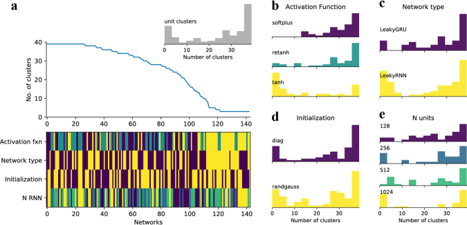
Extended Data Fig. 4 Activation function dictates whether clusters emerge in a network. A total of 144 networks were trained, each with different hyperparameters. (a) top: Networks are sorted by their numbers of clusters. bottom: the hyperparameters used for each network are indicated by colors, as defined in b-e. Inset, the distribution of cluster numbers across all networks. (b-e) Breaking down the number of clusters according to the (b) activation function (c) network architecture (d) weight initialization (e) number of units. Only networks that reached the minimum performance of 80% for every task are shown.
Extended Data Fig. 4 Activation function dictates whether clusters emerge in a network. A total of 144 networks were trained, each with different hyperparameters. (a) top: Networks are sorted by their numbers of clusters. bottom: the hyperparameters used for each network are indicated by colors, as defined in b-e. Inset, the distribution of cluster numbers across all networks. (b-e) Breaking down the number of clusters according to the (b) activation function (c) network architecture (d) weight initialization (e) number of units. Only networks that reached the minimum performance of 80% for every task are shown.CC BY · PubMed Central
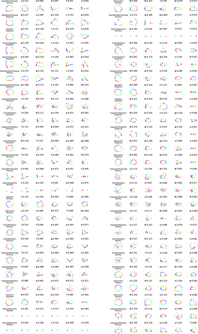
Extended Data Fig. 5 Qualitative structure and quantitative variance of the fixed points in each unit cluster. For each task period, we identified the fixed point most proximal to the network state at the end of the task period for thirty-two different input conditions. Fixed points most proximal to the network state were selected to focus our analysis on the most relevant fixed points for each task period. This analysis resulted in identification of thirty-two relevant fixed points for each task period that span stimulus conditions. We visualized the projection of these thirty-two fixed points in the top 2 PCs of the activity of all units (column 1) and in the top 2 PCs each unit cluster’s activity (column 2–6, letters denote unit cluster identity as in Fig. 3a). Due to space constraints, we visualize qualitative projections and quantification of variance for only the top 5 unit clusters, which capture maximal variance for each task period. In general, the rest of the unit clusters not shown captured less than 10% of the total variance each. For clusters with only one unit, we visualized this projection in one dimension (cluster x). Unit cluster identification (letters a-z) and normalized variance across fixed points projected into the space of all units within the cluster indicated above each visualization. We normalized variance by the sum of variance across all clusters. Rows are presented in the same order as the variance matrix for comparison (Fig. 3a).
Extended Data Fig. 5 Qualitative structure and quantitative variance of the fixed points in each unit cluster. For each task period, we identified the fixed point most proximal to the network state at the end of the task period for thirty-two different input conditions. Fixed points most proximal to the network state were selected to focus our analysis on the most relevant fixed points for each task period. This analysis resulted in identification of thirty-two relevant fixed points for each task period that span stimulus conditions. We visualized the projection of these thirty-two fixed points in the top 2 PCs of the activity of all units (column 1) and in the top 2 PCs each unit cluster’s activity (column 2–6, letters denote unit cluster identity as in Fig. 3a). Due to space constraints, we visualize qualitative projections and quantification of variance for only the top 5 unit clusters, which capture maximal variance for each task period. In general, the rest of the unit clusters not shown captured less than 10% of the total variance each. For clusters with only one unit, we visualized this projection in one dimension (cluster x). Unit cluster identification (letters a-z) and normalized variance across fixed points projected into the space of all units within the cluster indicated above each visualization. We normalized variance by the sum of variance across all clusters. Rows are presented in the same order as the variance matrix for comparison (Fig. 3a).CC BY · PubMed Central
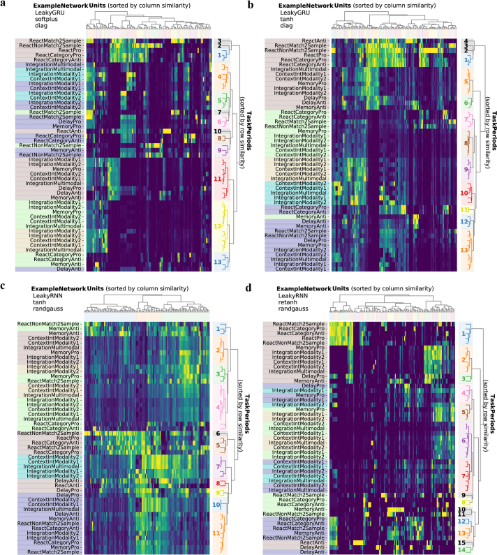
Extended Data Fig. 6 Example variance matrices for four different networks. Variance matrix for four example networks. Variance of unit activations across stimulus conditions, normalized across task periods (columns normalized by the maximum entry in each column). Rows and columns sorted according to similarity. Colors along left side label each task period type (dark blue: initial stimulus, light blue: second stimulus, light green: initial memory, yellow: second memory, brown: response). Notice blocks with high variance belong to same task period types (similar colors). Colors along the right side highlight task periods that were grouped together in clusters according to the optimal distance threshold for each dendrogram by computing the silhouette score based on intracluster and intercluster distances (see Clusters in Methods). (a) LeakyGRU, softplus, diagonal initialization, Nrec = 128 (b) LeakyGRU, tanh, diagonal initialization, Nrec = 128 (c) LeakyRNN, tanh, random Gaussian initialization, Nrec = 128 (d) LeakyRNN, retanh, random Gaussian initialization, Nrec = 128.
Extended Data Fig. 6 Example variance matrices for four different networks. Variance matrix for four example networks. Variance of unit activations across stimulus conditions, normalized across task periods (columns normalized by the maximum entry in each column). Rows and columns sorted according to similarity. Colors along left side label each task period type (dark blue: initial stimulus, light blue: second stimulus, light green: initial memory, yellow: second memory, brown: response). Notice blocks with high variance belong to same task period types (similar colors). Colors along the right side highlight task periods that were grouped together in clusters according to the optimal distance threshold for each dendrogram by computing the silhouette score based on intracluster and intercluster distances (see Clusters in Methods). (a) LeakyGRU, softplus, diagonal initialization, Nrec = 128 (b) LeakyGRU, tanh, diagonal initialization, Nrec = 128 (c) LeakyRNN, tanh, random Gaussian initialization, Nrec = 128 (d) LeakyRNN, retanh, random Gaussian initialization, Nrec = 128.CC BY · PubMed Central
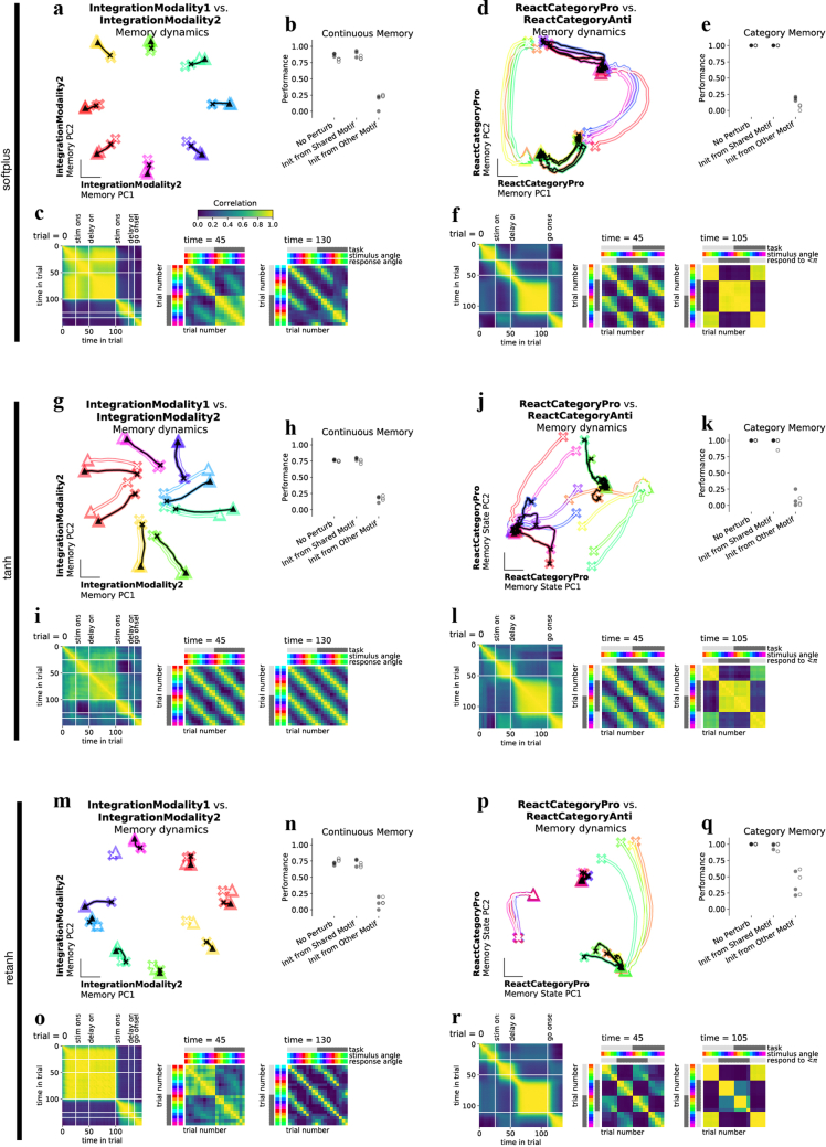
Extended Data Fig. 7 Discrete and continuous variable memory computations result in two kinds of shared memory attractors. We utilize analyses that could be performed in biological neural data or through behavioral experiments to highlight shared category and continuous memory dynamical motifs in networks with different activation functions. Networks were trained with softplus activation function for a-f (a) Neural state trajectories for eight stimulus conditions (colored by response direction) starting from ‘x’ in IntegrationModality2 PC space for IntegrationModality1 (white) and IntegrationModality2 (black) tasks. (b) Perturb initial condition for IntegrationModality1 response period state to the memory period final state of either IntegrationModality2 task (Init from shared motif), ReactCategoryAnti (Init from other motif) or IntegrationModality1 (No perturb) for trials with the same response direction and run the network forward through the response period. One data point for each of three networks trained with diagonal initialization (filled circles) or with a random Gaussian initialization (open circles). Performance was similar across ‘No perturb’ and ‘Init from shared motif’ conditions, but was dramatically impaired for ‘Init from other motif’ conditions. (c) left: Correlation across timesteps throughout an IntegrationModality1 trial. Task period transitions highlighted in white lines. middle: Correlation across trials for different stimulus conditions for IntegrationModality1 and IntegrationModality2 tasks at the end of the first stimulus period. right: Correlation across trials for different stimulus conditions for IntegrationModality1 and IntegrationModality2 tasks at the end of the memory period. Trials are highly correlated across tasks according to response direction. (d) Same as a for two category memory tasks, ReactCategoryPro (white) and ReactCategoryAnti (black). (e) Perturb initial condition for ReactCategoryPro response period state to the memory period final state of ReactCategoryAnti task (Init from shared motif), IntegrationModality1 (Init from other motif) or ReactCategoryPro (No perturb) for trials with the same response direction and run the network forward through the response period. (f) left: Correlation across timesteps throughout an ReactCategoryPro trial. Task period transitions highlighted in white lines. middle: Correlation across trials for different stimulus conditions for ReactCategoryPro and ReactCategoryAnti tasks at the end of the stimulus period. right: Correlation across trials for different stimulus conditions for ReactCategoryPro and ReactCategoryAnti tasks at the end of the memory period. Trials are highly correlated across tasks according to response direction. (g-l) Same as a-f for tanh activation function. (m-r) Same as a-f for retanh activation function. One example network in panels a,c,d,f (softplus activation), g,i,j,l (tanh activation) and m,o,p,r (retanh activation) where all three example networks have hyperparameters: LeakyRNN, 128 units, diagonal initialization.
Extended Data Fig. 7 Discrete and continuous variable memory computations result in two kinds of shared memory attractors. We utilize analyses that could be performed in biological neural data or through behavioral experiments to highlight shared category and continuous memory dynamical motifs in networks with different activation functions. Networks were trained with softplus activation function for a-f (a) Neural state trajectories for eight stimulus conditions (colored by response direction) starting from ‘x’ in IntegrationModality2 PC space for IntegrationModality1 (white) and IntegrationModality2 (black) tasks. (b) Perturb initial condition for IntegrationModality1 response period state to the memory period final state of either IntegrationModality2 task (Init from shared motif), ReactCategoryAnti (Init from other motif) or IntegrationModality1 (No perturb) for trials with the same response direction and run the network forward through the response period. One data point for each of three networks trained with diagonal initialization (filled circles) or with a random Gaussian initialization (open circles). Performance was similar across ‘No perturb’ and ‘Init from shared motif’ conditions, but was dramatically impaired for ‘Init from other motif’ conditions. (c) left: Correlation across timesteps throughout an IntegrationModality1 trial. Task period transitions highlighted in white lines. middle: Correlation across trials for different stimulus conditions for IntegrationModality1 and IntegrationModality2 tasks at the end of the first stimulus period. right: Correlation across trials for different stimulus conditions for IntegrationModality1 and IntegrationModality2 tasks at the end of the memory period. Trials are highly correlated across tasks according to response direction. (d) Same as a for two category memory tasks, ReactCategoryPro (white) and ReactCategoryAnti (black). (e) Perturb initial condition for ReactCategoryPro response period state to the memory period final state of ReactCategoryAnti task (Init from shared motif), IntegrationModality1 (Init from other motif) or ReactCategoryPro (No perturb) for trials with the same response direction and run the network forward through the response period. (f) left: Correlation across timesteps throughout an ReactCategoryPro trial. Task period transitions highlighted in white lines. middle: Correlation across trials for different stimulus conditions for ReactCategoryPro and ReactCategoryAnti tasks at the end of the stimulus period. right: Correlation across trials for different stimulus conditions for ReactCategoryPro and ReactCategoryAnti tasks at the end of the memory period. Trials are highly correlated across tasks according to response direction. (g-l) Same as a-f for tanh activation function. (m-r) Same as a-f for retanh activation function. One example network in panels a,c,d,f (softplus activation), g,i,j,l (tanh activation) and m,o,p,r (retanh activation) where all three example networks have hyperparameters: LeakyRNN, 128 units, diagonal initialization.CC BY · PubMed Central
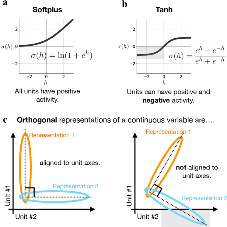
Extended Data Fig. 8 Positive activation functions align orthogonal motifs to unit axes. (a) softplus activation function maps activity to the positive real line. (b) tanh activation function does not impose positivity constraints. (c) left: Two activity patterns that are constrained to lie in the positive orthant can only be orthogonal to one another when aligned to the unit axes or with elevated activity levels (which is penalized as a biological constraint). right: Activation functions that result in positive or negative activity do not constrain activity patterns to unit axes. Note: Either system can use additional dimensions to orthogonalize representations not aligned to unit axes in an infinitely large network.
Extended Data Fig. 8 Positive activation functions align orthogonal motifs to unit axes. (a) softplus activation function maps activity to the positive real line. (b) tanh activation function does not impose positivity constraints. (c) left: Two activity patterns that are constrained to lie in the positive orthant can only be orthogonal to one another when aligned to the unit axes or with elevated activity levels (which is penalized as a biological constraint). right: Activation functions that result in positive or negative activity do not constrain activity patterns to unit axes. Note: Either system can use additional dimensions to orthogonalize representations not aligned to unit axes in an infinitely large network.CC BY · PubMed Central
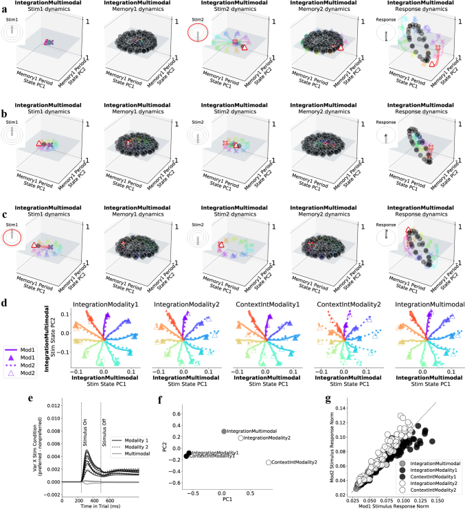
Extended Data Fig. 9 Integration tasks implement memory on a plane attractor; with stimulus processing through fixed points and contextual input amplification. Here we present fixed point structures and context dependent input responses for integration of a noisy continuous variable. (a-c) Fixed points and state trajectories during the multimodal integration task in one example network trained to perform all fifteen tasks. (a) All panels are different task periods from one trial where the first stimulus has a small amplitude, pointing upward and the second stimulus has a large amplitude pointing downward in both modality1 and modality2. Fixed points and state trajectories projected into PC space defined by state trajectories during the memory period of the IntegrationMultimodal task. Insets show stimulus direction and amplitude for both modalities: small amplitude stimuli reach the inner circle and large amplitude stimuli reach the outer circle. Large amplitude stimulus periods highlighted in red. From left to right panels: small amplitude input during first stimulus presentation produces dynamics that lack stable fixed point, resulting in the state remaining near initial condition. Memory period inputs result in a plane of marginally stable fixed points that maintain the position of the state after stimulus period 1. Stimulus period 2 has a large amplitude stimulus input, resulting in a single stable fixed point that attracts the state. The second memory period has the same inputs as the first memory period and therefore results in the same plane of marginally stable fixed points that maintain the position of the state after stimulus period 2. The response period inputs result in a ring of fixed points in output potent space that attracts the state to a region on the ring, dependent on initial conditions at the beginning of the response period (end of the memory period). Inset shows target output direction in thick gray line and actual outputs in thin black line emanating from ‘x’ and ending with ‘▴.’ Network correctly responds in the downward direction. (b) Same as a during one trial where first and second stimuli have medium amplitude. Identical amplitude inputs mean correct response direction is chosen at random. Network responds weakly downward. (c) Same as a during one trial where first stimulus has a large amplitude, pointing upward and the second stimulus has a small amplitude pointing downward. Network correctly responds upward. These panels demonstrate how fixed points guide the network to perform an integration task. (d) Demonstration of contextual input amplification for context dependent integration tasks. Stimulus dependent network state for both modality 1 (solid) and 2 (dotted) for five different tasks where relevant modality is specified in title for each subpanel. During IntegrationModality1 and IntegrationModality2 tasks, only the relevant stimulus is presented, but here we present either to compare state trajectories for each stimulus condition across tasks. Notice for contextual integration tasks, the state moves a greater distance from the origin in response to the relevant modality; whereas in the multimodal task, responses are fairly equal. (e) Quantification of contextual differences in d: Difference between variance across stimulus conditions for preferred modality minus variance across stimulus conditions for nonpreferred modality. Preference is defined by task rules. One line for each of five tasks in three different networks with different random seeds. (f) Context period network state for all five tasks projected onto the first and second PCs defined by variance of the state across tasks at the end of the context period (PCA on 5 × Nrec matrix). Organization of network states at the end of the context period shows compositional structure. PC1 goes from modality 1- > 2 and PC2 separates ContextIntegration vs. Integration decision tasks. (g) Norm of input response for twenty-four stimulus conditions spanning [0, 2π) on each of five tasks (see Effective input modulation Methods). Trials where the network should prefer Modality 1 are black, Modality 2 white, multimodal gray. It will be an interesting direction for future work to determine whether other features of the dynamics, such as input response amplification, could be shared across contexts in a similar manner to how fixed points are shared. This could be done through interpolation of initial conditions with identical inputs. Hyperparameters: LeakyRNN, softplus activation, diagonal initialization, Nrec = 128.
Extended Data Fig. 9 Integration tasks implement memory on a plane attractor; with stimulus processing through fixed points and contextual input amplification. Here we present fixed point structures and context dependent input responses for integration of a noisy continuous variable. (a-c) Fixed points and state trajectories during the multimodal integration task in one example network trained to perform all fifteen tasks. (a) All panels are different task periods from one trial where the first stimulus has a small amplitude, pointing upward and the second stimulus has a large amplitude pointing downward in both modality1 and modality2. Fixed points and state trajectories projected into PC space defined by state trajectories during the memory period of the IntegrationMultimodal task. Insets show stimulus direction and amplitude for both modalities: small amplitude stimuli reach the inner circle and large amplitude stimuli reach the outer circle. Large amplitude stimulus periods highlighted in red. From left to right panels: small amplitude input during first stimulus presentation produces dynamics that lack stable fixed point, resulting in the state remaining near initial condition. Memory period inputs result in a plane of marginally stable fixed points that maintain the position of the state after stimulus period 1. Stimulus period 2 has a large amplitude stimulus input, resulting in a single stable fixed point that attracts the state. The second memory period has the same inputs as the first memory period and therefore results in the same plane of marginally stable fixed points that maintain the position of the state after stimulus period 2. The response period inputs result in a ring of fixed points in output potent space that attracts the state to a region on the ring, dependent on initial conditions at the beginning of the response period (end of the memory period). Inset shows target output direction in thick gray line and actual outputs in thin black line emanating from ‘x’ and ending with ‘▴.’ Network correctly responds in the downward direction. (b) Same as a during one trial where first and second stimuli have medium amplitude. Identical amplitude inputs mean correct response direction is chosen at random. Network responds weakly downward. (c) Same as a during one trial where first stimulus has a large amplitude, pointing upward and the second stimulus has a small amplitude pointing downward. Network correctly responds upward. These panels demonstrate how fixed points guide the network to perform an integration task. (d) Demonstration of contextual input amplification for context dependent integration tasks. Stimulus dependent network state for both modality 1 (solid) and 2 (dotted) for five different tasks where relevant modality is specified in title for each subpanel. During IntegrationModality1 and IntegrationModality2 tasks, only the relevant stimulus is presented, but here we present either to compare state trajectories for each stimulus condition across tasks. Notice for contextual integration tasks, the state moves a greater distance from the origin in response to the relevant modality; whereas in the multimodal task, responses are fairly equal. (e) Quantification of contextual differences in d: Difference between variance across stimulus conditions for preferred modality minus variance across stimulus conditions for nonpreferred modality. Preference is defined by task rules. One line for each of five tasks in three different networks with different random seeds. (f) Context period network state for all five tasks projected onto the first and second PCs defined by variance of the state across tasks at the end of the context period (PCA on 5 × Nrec matrix). Organization of network states at the end of the context period shows compositional structure. PC1 goes from modality 1- > 2 and PC2 separates ContextIntegration vs. Integration decision tasks. (g) Norm of input response for twenty-four stimulus conditions spanning [0, 2π) on each of five tasks (see Effective input modulation Methods). Trials where the network should prefer Modality 1 are black, Modality 2 white, multimodal gray. It will be an interesting direction for future work to determine whether other features of the dynamics, such as input response amplification, could be shared across contexts in a similar manner to how fixed points are shared. This could be done through interpolation of initial conditions with identical inputs. Hyperparameters: LeakyRNN, softplus activation, diagonal initialization, Nrec = 128.CC BY · PubMed Central
Extended Data Fig. 10 Leave-one-out transfer learning is possible through reuse of previously learned motifs and is therefore less effective for tasks with unique dynamical motifs. (a-d) Performance during training single rule input weights for (a) MemoryAnti (b) IntegrationMultimodal (c) ReactMatch2Sample and (d) ReactAnti tasks after pre-training all other weights and biases on all other tasks (black) and during training all weights and biases on a single rule (gray, 3 lines for 3 different networks with different random reeds). Single task networks provide a baseline comparison to measure how well the transfer learning method works for any given task. Notice transfer learning method typically results in faster learning (black line goes up before grey lines), except for ReactAnti task, which is rapidly learned in both cases. During training of the ReactMatch2Sample tasks, single task networks with fully plastic weights eventually out-perform transfer learning networks with only one plastic input. Through examination of the similarity of unit activations across tasks, we understand single task networks’ superiority over the transfer learning method to be a result of unique dynamical motifs in the held-out task (ReactMatch2Sample). (e) left: Performance early in training novel task for single task networks (dot) and transfer learning network (arrowhead) (as in a-d) plotted against task period max correlation (for a given task, plotting task period with the highest max correlation with other rows in the variance matrix, Fig. 3a). Task period max correlation was averaged across networks with all hyperparameter settings in Fig. 3b (see Transfer learning Methods for details). High correlation values on the x-axis highlight that all tasks (except ReactAnti) have at least one task period with high correlation (>.5) to a task period from a different task, and therefore benefit from pre-training to some extent (arrowhead above dot in all cases). Some tasks are so easy (DelayPro, DelayAnti, ReactPro and ReactAnti) that performance is nearly 100% in both transfer learning and single task networks at the early training step, resulting in zero performance difference. right: Performance difference (transfer learning performance - single task network performance) late in learning plotted against task period max correlation for the task period with the lowest value in each task. The x-axis shows which tasks include task periods with novel dynamical motifs indicated by low correlation to task periods in other tasks (for a given task, plotting task period with the lowest max correlation with other rows in the variance matrix, Fig. 3a). (f-g) Same as e for other single task networks with different random seeds. ReactMatch2Sample and ReactNonMatch2Sample tasks both have a task period with low correlation to other task periods from different tasks and therefore ReactMatch2Sample and ReactNonMatch2Sample tasks require unique dynamical motifs. Those were the same tasks where single task learning outperformed the transfer learning approach. This suggests our transfer learning approach depends on pre-training necessary motifs. (h-k) Additional support that leave-one-out transfer learning is possible through reuse of previously learned motifs: These figures present additional support for examples in the main text (Fig. 6). We first train on all tasks except ContextIntegrationModality2 and then use our transfer learning approach to learn the context inputs for the held-out task. Same stimulus fixed point was reused across ContextIntegrationModality1 and 2 tasks. Memory period reused the same plane attractor to store the amplitude information of the stimulus. See Extended Data Fig. 9 for detailed fixed-point structures on the integration tasks. Input interpolation between fixed points across ContextIntegrationModality1 and ContextIntegrationModality2 tasks during (h-i) ‘Stimulus Integration’ and (j-k) ‘Integration Memory’ motifs for (h) Rule input interpolation across context integration tasks for one stimulus angle during first stimulus period. middle: Unstable (open) and stable (closed) fixed points for 20 intermediate α values (x-axis) projected onto top two PCs defined by state trajectories during the stimulus period both tasks concatenated (y and z-axes) with (left) ContextIntegrationModality2 α=0 and (right) ContextIntegrationModality1 α=1 fixed points and trajectories for 8 different stimulus angles (rainbow colors). (i) left: Maximum real eigenvalue for the linearization of the state update around each fixed point single fixed point closest to the state at the end of the stimulus period for 20 consecutive α values between 0 and 1. right: Euclidean distance between consecutive fixed points in the full state space (blue), outside of the visualized subspace in h (orange) and within the visualized space (green). We analyzed only one fixed point that is most proximal to the end of the state trajectory for each input condition to highlight the task relevant fixed point (see Analysis of fixed points for interpolated inputs in Methods). (j-k) Same as h-i, but for memory period. Panels h-k generated from the same network. All networks in a-g were trained with the same hyperparameters: LeakyRNN, softplus activation, diagonal initialization, Nrec = 128 for transfer learning and single task networks.
Extended Data Fig. 10 Leave-one-out transfer learning is possible through reuse of previously learned motifs and is therefore less effective for tasks with unique dynamical motifs. (a-d) Performance during training single rule input weights for (a) MemoryAnti (b) IntegrationMultimodal (c) ReactMatch2Sample and (d) ReactAnti tasks after pre-training all other weights and biases on all other tasks (black) and during training all weights and biases on a single rule (gray, 3 lines for 3 different networks with different random reeds). Single task networks provide a baseline comparison to measure how well the transfer learning method works for any given task. Notice transfer learning method typically results in faster learning (black line goes up before grey lines), except for ReactAnti task, which is rapidly learned in both cases. During training of the ReactMatch2Sample tasks, single task networks with fully plastic weights eventually out-perform transfer learning networks with only one plastic input. Through examination of the similarity of unit activations across tasks, we understand single task networks’ superiority over the transfer learning method to be a result of unique dynamical motifs in the held-out task (ReactMatch2Sample). (e) left: Performance early in training novel task for single task networks (dot) and transfer learning network (arrowhead) (as in a-d) plotted against task period max correlation (for a given task, plotting task period with the highest max correlation with other rows in the variance matrix, Fig. 3a). Task period max correlation was averaged across networks with all hyperparameter settings in Fig. 3b (see Transfer learning Methods for details). High correlation values on the x-axis highlight that all tasks (except ReactAnti) have at least one task period with high correlation (>.5) to a task period from a different task, and therefore benefit from pre-training to some extent (arrowhead above dot in all cases). Some tasks are so easy (DelayPro, DelayAnti, ReactPro and ReactAnti) that performance is nearly 100% in both transfer learning and single task networks at the early training step, resulting in zero performance difference. right: Performance difference (transfer learning performance - single task network performance) late in learning plotted against task period max correlation for the task period with the lowest value in each task. The x-axis shows which tasks include task periods with novel dynamical motifs indicated by low correlation to task periods in other tasks (for a given task, plotting task period with the lowest max correlation with other rows in the variance matrix, Fig. 3a). (f-g) Same as e for other single task networks with different random seeds. ReactMatch2Sample and ReactNonMatch2Sample tasks both have a task period with low correlation to other task periods from different tasks and therefore ReactMatch2Sample and ReactNonMatch2Sample tasks require unique dynamical motifs. Those were the same tasks where single task learning outperformed the transfer learning approach. This suggests our transfer learning approach depends on pre-training necessary motifs. (h-k) Additional support that leave-one-out transfer learning is possible through reuse of previously learned motifs: These figures present additional support for examples in the main text (Fig. 6). We first train on all tasks except ContextIntegrationModality2 and then use our transfer learning approach to learn the context inputs for the held-out task. Same stimulus fixed point was reused across ContextIntegrationModality1 and 2 tasks. Memory period reused the same plane attractor to store the amplitude information of the stimulus. See Extended Data Fig. 9 for detailed fixed-point structures on the integration tasks. Input interpolation between fixed points across ContextIntegrationModality1 and ContextIntegrationModality2 tasks during (h-i) ‘Stimulus Integration’ and (j-k) ‘Integration Memory’ motifs for (h) Rule input interpolation across context integration tasks for one stimulus angle during first stimulus period. middle: Unstable (open) and stable (closed) fixed points for 20 intermediate α values (x-axis) projected onto top two PCs defined by state trajectories during the stimulus period both tasks concatenated (y and z-axes) with (left) ContextIntegrationModality2 α=0 and (right) ContextIntegrationModality1 α=1 fixed points and trajectories for 8 different stimulus angles (rainbow colors). (i) left: Maximum real eigenvalue for the linearization of the state update around each fixed point single fixed point closest to the state at the end of the stimulus period for 20 consecutive α values between 0 and 1. right: Euclidean distance between consecutive fixed points in the full state space (blue), outside of the visualized subspace in h (orange) and within the visualized space (green). We analyzed only one fixed point that is most proximal to the end of the state trajectory for each input condition to highlight the task relevant fixed point (see Analysis of fixed points for interpolated inputs in Methods). (j-k) Same as h-i, but for memory period. Panels h-k generated from the same network. All networks in a-g were trained with the same hyperparameters: LeakyRNN, softplus activation, diagonal initialization, Nrec = 128 for transfer learning and single task networks.CC BY · PubMed Central

Verification

Claims the paper makes

The claims and statistics of this paper haven’t been checked yet.

Run the check — free, no account needed. It reads the open-access text and checks the sources it cites.

A few free checks a day · papers already verified open instantly · results are public

Claims other papers make about this one

Each is checked against this paper’s own text: does it say what the citing paper says it does?

Self-check

Percentages, sums and reported differences re-computed from the paper’s own numbers.

The self-check needs the paper’s full text.

Citations

Cites

Show all 62 references

Research works printed but not linked: 5

  1. 1989, in Psychology of Learning and Motivation, 24, 109
  2. Goudar, V. , Peysakhovich, B. , Freedman, D. J. & Buffalo, E. A. Elucidating the neural mechanisms of Learning-to-Learn. bioRxiv (2021).
  3. 2019, Task representations in neural networks trained to perform many cognitive tasks, Nature neuroscience, 22, 297, 10.1038/s41593-018-0310-2 · DOI · Paper page
  4. 2018, Fixedpoint?nder: A tensor?ow toolbox for identifying and characterizing ?xed points in recurrent neural networks, Journal of Open Source Software, 3, 1003, 10.21105/joss.01003 · DOI
  5. 10.1038/nature12742 · DOI

Cited by

Sorted by citations

Metadata

Authors
Driscoll, L., Shenoy, K., & Sussillo, D.
Affiliations
  • Stanford University (US)
  • Howard Hughes Medical Institute (US)
Corresponding author
Driscoll, Laura
Venue
Nature Neuroscience
Publisher
openRxiv
Published
2022-08-15
Volume
27
Issue
7
Pages
1349-1363
ISSN
1097-6256 (ISSN-L)
OpenAlex
W4400462656
Cited by
217
References
62
Citations by year
2026: 78 · 2025: 58 · 2024: 45 · 2023: 31 · 2022: 4
FWCI
26.71
Type
journal article
Language
en
Open access
Licence
cc-by
Locations
  • Nature Neuroscience (publishedVersion, cc-by)
  • bioRxiv (Cold Spring Harbor Laboratory) (acceptedVersion)
  • PubMed Central (publishedVersion, cc-by)
  • PubMed (publishedVersion)
Funders
Simons Foundation (543049, 1155867, 543045)
Topics
  • Physical Sciences › Computer Science › Artificial Intelligence › Neural Networks and Applications
  • Life Sciences › Neuroscience › Cognitive Neuroscience › Neural dynamics and brain function
  • Life Sciences › Neuroscience › Cognitive Neuroscience › Memory and Neural Mechanisms
Keywords
recurrent neural networks, multi-task learning, modular computation, ring attractor, attractor dynamics, decision boundaries, transfer learning
MeSH terms
Algorithms, Animals, Learning, Models, Neurological, Nerve Net, Neurons, Neural Networks, Computer

About these checks

Registry, retraction, Cites and statistics results are computed, not judged, with one exception: a printed reference that no index lists is read once by a model before it counts as a citation error. Claims are extracted by a model and kept only when their quote appears verbatim in the text; each cited source is then checked, with a model’s help, for whether it says what the claim relies on. Those verdicts can be wrong — read the claim’s quote and the cited source before relying on one.

Statistics and arithmetic are recomputed, not judged.

Confidence bands are shown only for fields calibrated on our annotated test set. None is calibrated yet, so no band is shown.

What counts as a claim ›How we measure confidence ›How we check this ›

Are you an author, or do you see a problem with this page? Request a review