

The DOI matches its Crossref record; 67 of the 72 references it cites were found in a registry or an index.
Automated model building and protein identification in cryo-EM maps
Open accessPreprint — published as 10.1038/s41586-024-07215-4 · Paper page
Abstract
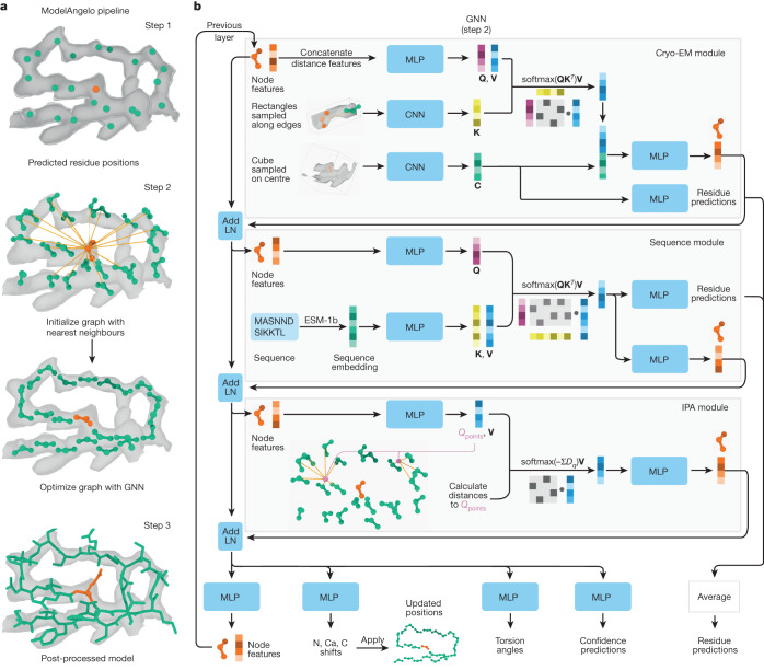
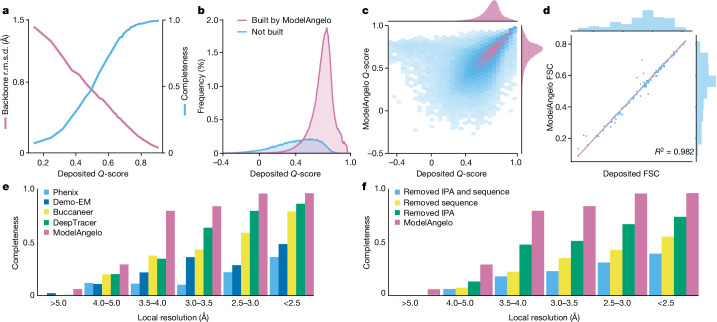
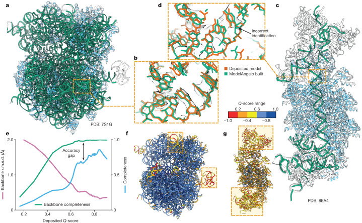
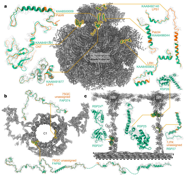
Interpreting electron cryo-microscopy (cryo-EM) maps with atomic models requires high levels of expertise and labour-intensive manual intervention. We present ModelAngelo, a machine-learning approach for automated atomic model building in cryo-EM maps. By combining information from the cryo-EM map with information from protein sequence and structure in a single graph neural network, ModelAngelo builds atomic models for proteins that are of similar quality as those generated by human experts. For nucleotides, ModelAngelo builds backbones with similar accuracy as humans. By using its predicted amino acid probabilities for each residue in hidden Markov model sequence searches, ModelAngelo outperforms human experts in the identification of proteins with unknown sequences. ModelAngelo will thus remove bottlenecks and increase objectivity in cryo-EM structure determination.
Overview
The claims and statistics of this paper haven’t been checked yet.
Run the check — free, no account needed. It reads the open-access text and checks the sources it cites.
Integrity signals
Registry
Cites
Statistics
Figures
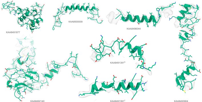
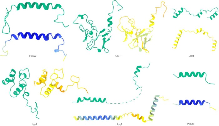
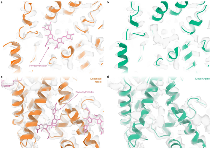
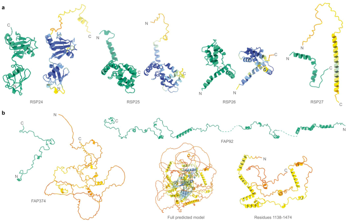
Verification
Claims the paper makes
The claims and statistics of this paper haven’t been checked yet.
Run the check — free, no account needed. It reads the open-access text and checks the sources it cites.
Self-check
Percentages, sums and reported differences re-computed from the paper’s own numbers.
The self-check needs the paper’s full text.
Citations
Cites
Deep Residual Learning for Image Recognition
He, K., Zhang, X., Ren, S., & Sun, J. (2016) · 2016 IEEE Conference on Computer Vision and Pattern Recognition (CVPR) · doi:10.1109/cvpr.2016.90 · Cited by 235,474
Vaswani, A., Shazeer, N., Parmar, N., Uszkoreit, J., Jones, L., Gomez, A. N., Kaiser, L., & Polosukhin, I. (2017) · arXiv · doi:10.48550/arxiv.1706.03762 · Cited by 120,404
Highly accurate protein structure prediction with AlphaFold
Jumper, J., Evans, R., Pritzel, A., Green, T., Figurnov, M., Ronneberger, O., Tunyasuvunakool, K., Bates, R., Žídek, A., Potapenko, A., et al. (2021) · Nature · doi:10.1038/s41586-021-03819-2 · Cited by 43,764
Feature Pyramid Networks for Object Detection
Lin, T.-Y., Dollar, P., Girshick, R., He, K., Hariharan, B., & Belongie, S. (2017) · 2017 IEEE Conference on Computer Vision and Pattern Recognition (CVPR) · doi:10.1109/cvpr.2017.106 · Cited by 30,939
Features and development of Coot
Emsley, P., Lohkamp, B., Scott, W. G., & Cowtan, K. (2010) · Acta Crystallographica Section D Biological Crystallography · doi:10.1107/s0907444910007493 · Cited by 29,915
Mfold web server for nucleic acid folding and hybridization prediction
Zuker, M. (2003) · Nucleic Acids Research · doi:10.1093/nar/gkg595 · Cited by 13,404
ColabFold - Making protein folding accessible to all
Mirdita, M., Schütze, K., Moriwaki, Y., Heo, L., Ovchinnikov, S., & Steinegger, M. (2021) · doi:10.1101/2021.08.15.456425 · Cited by 9,391
Liebschner, D., Afonine, P. V., Baker, M. L., Bunkóczi, G., Chen, V. B., Croll, T. I., Hintze, B., Hung, L.-W., Jain, S., McCoy, A. J., et al. (2019) · Acta Crystallographica Section D Structural Biology · doi:10.1107/s2059798319011471 · Cited by 7,953
Varadi, M., Anyango, S., Deshpande, M., Nair, S., Natassia, C., Yordanova, G., Yuan, D., Stroe, O., Wood, G., Laydon, A., et al. (2022) · Nucleic Acids Research · doi:10.1093/nar/gkab1061 · Cited by 7,850
Accelerated Profile HMM Searches
Eddy, S. R. (2011) · PLoS Computational Biology · doi:10.1371/journal.pcbi.1002195 · Cited by 6,975
Research works printed but not linked: 3
- 14. Lin, Z., et al. Language models of protein sequences at the scale of evolution enable accurate structure prediction. bioRxiv (2022). URL https://www.biorxiv.org/content/early/2022/07/21/2022.07.20.500902. https://www.biorxiv.org/content/early/2022/07/21/2022.07.20.500902.full.pdf.
- Jamali, K. , Kimanius, D. & Scheres, S. H . A graph neural network approach to automated model building in cryo-EM maps. In The Eleventh International Conference on Learning Representations (2023). URL https://openreview.net/forum?id=65XDF_nwI61.
- 2019, Macromolecular structure determination using x-rays, neutrons and electrons: recent developments in phenix, Acta Crystallographica Section D: Structural Biology, 75, 861, 10.1107/S2059798319011471 · DOI · Paper page
Cited by
Sorted by citations
An image processing pipeline for electron cryo‐tomography in RELION ‐5
Burt, A., Toader, B., Warshamanage, R., von Kügelgen, A., Pyle, E., Zivanov, J., Kimanius, D., Bharat, T. A. M., & Scheres, S. H. W. (2024) · FEBS Open Bio · doi:10.1002/2211-5463.13873 · Cited by 254
Self-citationTargeted protein degradation via intramolecular bivalent glues
Hsia, O., Hinterndorfer, M., Cowan, A. D., Iso, K., Ishida, T., Sundaramoorthy, R., Nakasone, M. A., Imrichova, H., Schätz, C., Rukavina, A., et al. (2024) · Nature · doi:10.1038/s41586-024-07089-6 · Cited by 222
Disease-specific tau filaments assemble via polymorphic intermediates
Lövestam, S., Li, D., Wagstaff, J. L., Kotecha, A., Kimanius, D., McLaughlin, S. H., Murzin, A. G., Freund, S. M. V., Goedert, M., & Scheres, S. H. W. (2023) · Nature · doi:10.1038/s41586-023-06788-w · Cited by 207
Self-citationEMDB—the Electron Microscopy Data Bank
Turner, J., Abbott, S., Fonseca, N., Pye, R., de Oliveira, L. C., Duraisamy, A. K., Salih, O., Wang, Z., Kleywegt, G. J., Morris, K. L., et al. (2023) · Nucleic Acids Research · doi:10.1093/nar/gkad1019 · Cited by 154
Structural specializations of the sperm tail
Leung, M. R., Zeng, J., Wang, X., Roelofs, M. C., Huang, W., Chiozzi, R. Z., Hevler, J. F., Heck, A. J. R., Dutcher, S. K., Brown, A., et al. (2023) · Cell · doi:10.1016/j.cell.2023.05.026 · Cited by 145
Self-citation
Metadata
- Authors
- Jamali, K., Käll, L., Zhang, R., Brown, A., Kimanius, D., & Scheres, S. H. W.
- Affiliations
- MRC Laboratory of Molecular Biology (GB)
- Science for Life Laboratory (SE)
- Washington University in St. Louis (US)
- Harvard University (US)
- Corresponding author
- Jamali, Kiarash
- Kimanius, Dari
- Scheres, Sjors H.W.
- Venue
- Nature
- Publisher
- openRxiv
- Published
- 2023-05-16
- Volume
- 628
- Issue
- 8007
- Pages
- 450-457
- ISSN
- 0028-0836 (ISSN-L)
- PMC
- PMC11006616
- OpenAlex
- W4392155415
- Cited by
- 686
- References
- 72
- Citations by year
- 2026: 259 · 2025: 264 · 2024: 134 · 2023: 28
- FWCI
- 120.08
- Type
- journal article
- Language
- en
- Open access
- hybrid
- doi.org
- Licence
- cc-by
- Locations
- Nature (publishedVersion, cc-by)
- bioRxiv (Cold Spring Harbor Laboratory) (acceptedVersion, cc-by)
- PubMed Central (publishedVersion, cc-by)
- PubMed (publishedVersion)
- Apollo (University of Cambridge) (acceptedVersion, cc-by)
- PubMed Central (submittedVersion, cc-by)
- Digital Commons@Becker (Washington University School of Medicine) (submittedVersion, cc-by)
- RePEc: Research Papers in Economics (submittedVersion)
- Zenodo (CERN European Organization for Nuclear Research) (submittedVersion, cc-by)
- Funders
- European Commission (HORIZON2020, 895412)
- Knut och Alice Wallenbergs Stiftelse (2022.0032)
- National Institutes of Health
- Medical Research Council (MC_UP_A025_1013)
- National Institute of General Medical Sciences (R01GM138854, R01GM141109)
- Topics
- Life Sciences › Biochemistry, Genetics and Molecular Biology › Structural Biology › Advanced Electron Microscopy Techniques and Applications
- Life Sciences › Biochemistry, Genetics and Molecular Biology › Molecular Biology › Protein Structure and Dynamics
- Life Sciences › Biochemistry, Genetics and Molecular Biology › Structural Biology › Enzyme Structure and Function
- Keywords
- cryo-EM density maps, protein identification, graph neural networks, protein structure determination, machine learning
About these checks
Registry, retraction, Cites and statistics results are computed, not judged, with one exception: a printed reference that no index lists is read once by a model before it counts as a citation error. Claims are extracted by a model and kept only when their quote appears verbatim in the text; each cited source is then checked, with a model’s help, for whether it says what the claim relies on. Those verdicts can be wrong — read the claim’s quote and the cited source before relying on one.
Statistics and arithmetic are recomputed, not judged.
Confidence bands are shown only for fields calibrated on our annotated test set. None is calibrated yet, so no band is shown.
What counts as a claim ›How we measure confidence ›How we check this ›
Are you an author, or do you see a problem with this page? Request a review
