

Low-overhead fault-tolerant quantum computing using long-range connectivity
Open accessThe DOI matches its Crossref record; 93 of the 93 references it cites were found in a registry or an index.
Abstract
Vast numbers of qubits will be needed for large-scale quantum computing because of the overheads associated with error correction. We present a scheme for low-overhead fault-tolerant quantum computation based on quantum low-density parity-check (LDPC) codes, where long-range interactions enable many logical qubits to be encoded with a modest number of physical qubits. In our approach, logic gates operate via logical Pauli measurements that preserve both the protection of the LDPC codes and the low overheads in terms of the required number of additional qubits. Compared with surface codes with the same code distance, we estimate order-of-magnitude improvements in the overheads for processing around 100 logical qubits using this approach. Given the high thresholds demonstrated by LDPC codes, our estimates suggest that fault-tolerant quantum computation at this scale may be achievable with a few thousand physical qubits at comparable error rates to what is needed for current approaches.
Overview
The claims and statistics of this paper haven’t been checked yet.
Free: it reads the open-access text and checks the first 5 claims that cite a source we can check. Create a free account to check every claim.
Integrity signals
Registry
Cites
Statistics
Figures
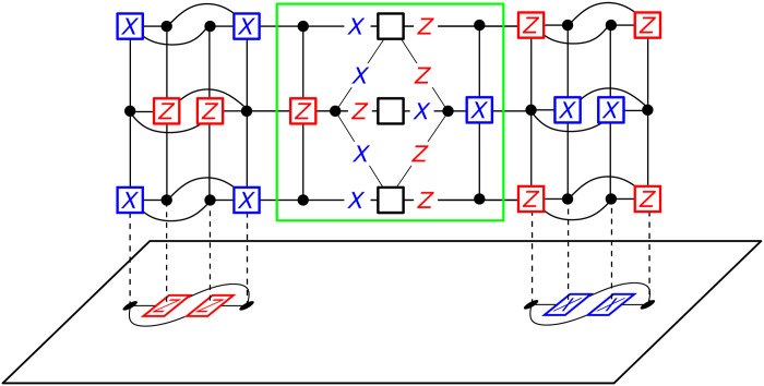
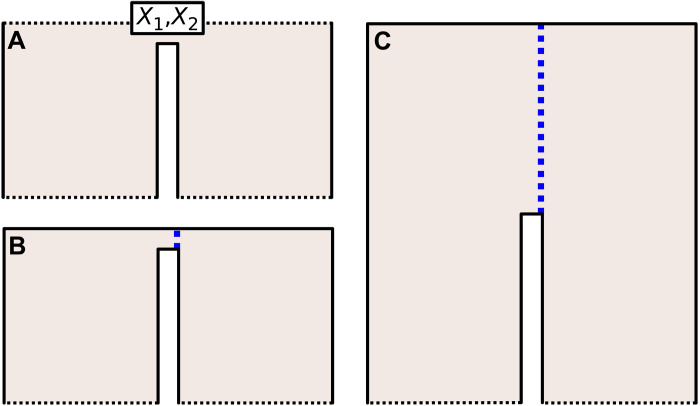
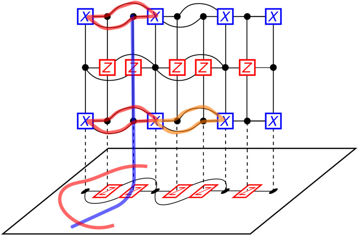
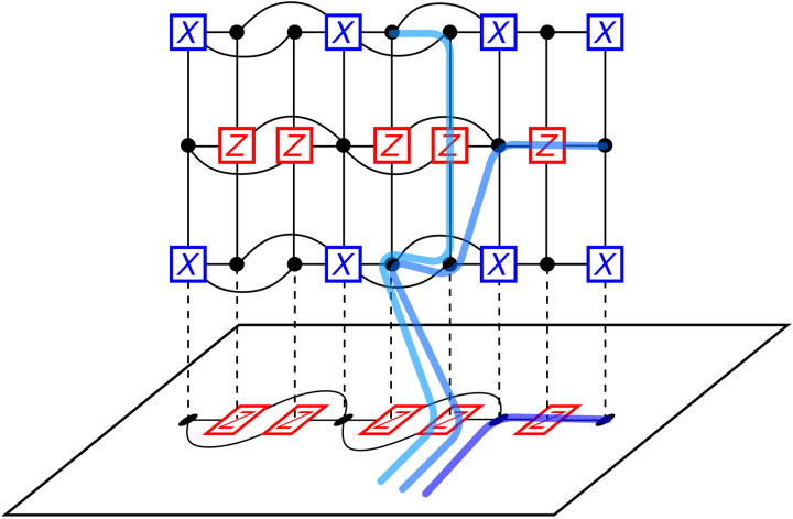
Verification
Claims the paper makes
The claims and statistics of this paper haven’t been checked yet.
Free: it reads the open-access text and checks the first 5 claims that cite a source we can check. Create a free account to check every claim.
Claims other papers make about this one
Each is checked against this paper’s own text: does it say what the citing paper says it does?
The cited source says what the claim attributes to it.
In the citing paper
“As shown in Fig. 1c, extensions of the Tanner graph leveraging techniques by Cohen et al.50 enable fault-tolerant measurement operations involving an ancillary surface code.”
From High-threshold and low-overhead fault-tolerant quantum memory (2024) · cites this paper as Cohen et al.50
Self-check
Percentages, sums and reported differences re-computed from the paper’s own numbers.
The self-check needs the paper’s full text.
Citations
Cites
Quantum supremacy using a programmable superconducting processor
Arute, F., Arya, K., Babbush, R., Bacon, D., Bardin, J. C., Barends, R., Biswas, R., Boixo, S., Brandao, F. G. S. L., Buell, D. A., et al. (2019) · Nature · doi:10.1038/s41586-019-1666-5 · Cited by 7,720
Fault-tolerant quantum computation by anyons
Kitaev, A. Y. (2003) · Annals of Physics · doi:10.1016/s0003-4916(02)00018-0 · Cited by 7,238
Surface codes: Towards practical large-scale quantum computation
Fowler, A. G., Mariantoni, M., Martinis, J. M., & Cleland, A. N. (2012) · Physical Review A · doi:10.1103/physreva.86.032324 · Cited by 3,059
Dennis, E., Kitaev, A., Landahl, A., & Preskill, J. (2002) · Journal of Mathematical Physics · doi:10.1063/1.1499754 · Cited by 1,768
Universal quantum computation with ideal Clifford gates and noisy ancillas
Bravyi, S., & Kitaev, A. (2005) · Physical Review A · doi:10.1103/physreva.71.022316 · Cited by 1,525 · cited 4×
“These logical operations then yield a universal gate set for fault-tolerant quantum computing when supplemented with noisy ancilla state injection via magic-state distillation [50].”
BackgroundMethodInfluentialDennis, E., Kitaev, A., Landahl, A., & Preskill, J. (2001) · CERN Document Server (European Organization for Nuclear Research) · Cited by 1,485
Hamiltonian Simulation by Qubitization
Low, G. H., & Chuang, I. L. (2019) · Quantum · doi:10.22331/q-2019-07-12-163 · Cited by 854
How to factor 2048 bit RSA integers in 8 hours using 20 million noisy qubits
Gidney, C., & Ekerå, M. (2021) · Quantum · doi:10.22331/q-2021-04-15-433 · Cited by 830
Fault-Tolerant Quantum Computation with High Threshold in Two Dimensions
Raussendorf, R., & Harrington, J. (2007) · Physical Review Letters · doi:10.1103/physrevlett.98.190504 · Cited by 812
Demonstration of a small programmable quantum computer with atomic qubits
Debnath, S., Linke, N. M., Figgatt, C., Landsman, K. A., Wright, K., & Monroe, C. (2016) · Nature · doi:10.1038/nature18648 · Cited by 777
Stabilizer Codes and Quantum Error Correction
Gottesman, D. (1997) · arXiv · doi:10.48550/arxiv.quant-ph/9705052 · Cited by 753
Elucidating reaction mechanisms on quantum computers
Reiher, M., Wiebe, N., Svore, K. M., Wecker, D., & Troyer, M. (2017) · Proceedings of the National Academy of Sciences · doi:10.1073/pnas.1619152114 · Cited by 745 · cited 5×
“The above argument tells us that we can shift qubits in VL̃[1] to VL̃[2] while creating non-trivial support on V T L̃ [1].”
BackgroundInfluentialHamiltonian Simulation by Qubitization
Low, G. H., & Chuang, I. L. (2019) · DSpace@MIT (Massachusetts Institute of Technology) · Cited by 714
Topological Quantum Distillation
Bombin, H., & Martin-Delgado, M. A. (2006) · Physical Review Letters · doi:10.1103/physrevlett.97.180501 · Cited by 700
Surface code quantum computing by lattice surgery
Horsman, D., Fowler, A. G., Devitt, S., & Meter, R. V. (2012) · New Journal of Physics · doi:10.1088/1367-2630/14/12/123011 · Cited by 598 · cited 4×
“Our method is a form of code deformation, in which we transform our code into a new code and in doing so obtain logical information about our original code [5, 13, 30, 41–43].”
BackgroundMethodInfluentialRealization of three-qubit quantum error correction with superconducting circuits
Reed, M. D., DiCarlo, L., Nigg, S. E., Sun, L., Frunzio, L., Girvin, S. M., & Schoelkopf, R. J. (2012) · Nature · doi:10.1038/nature10786 · Cited by 585
Demonstration of the trapped-ion quantum CCD computer architecture
Pino, J. M., Dreiling, J. M., Figgatt, C., Gaebler, J. P., Moses, S. A., Allman, M. S., Baldwin, C. H., Foss-Feig, M., Hayes, D., Mayer, K., et al. (2021) · Nature · doi:10.1038/s41586-021-03318-4 · Cited by 547 · cited 2×
“With long-range coupling now demonstrated us-ing a number of very different approaches [14–19], as well as proposals allowing all-to-all coupling [53], there is significant room for innovation here.”
BackgroundEfficient high-fidelity quantum computation using matter qubits and linear optics
Barrett, S. D., & Kok, P. (2005) · Physical Review A · doi:10.1103/physreva.71.060310 · Cited by 546
Operator quantum error-correcting subsystems for self-correcting quantum memories
Bacon, D. (2006) · Physical Review A · doi:10.1103/physreva.73.012340 · Cited by 486 · cited 1×
“[11] Dave Bacon, “Operator quantum error-correcting subsys-”
Entanglement distillation between solid-state quantum network nodes
Kalb, N., Reiserer, A. A., Humphreys, P. C., Bakermans, J. J. W., Kamerling, S. J., Nickerson, N. H., Benjamin, S. C., Twitchen, D. J., Markham, M., & Hanson, R. (2017) · Science · doi:10.1126/science.aan0070 · Cited by 413
A Game of Surface Codes: Large-Scale Quantum Computing with Lattice Surgery
Litinski, D. (2019) · Quantum · doi:10.22331/q-2019-03-05-128 · Cited by 408
Quantum computations on a topologically encoded qubit
Nigg, D., Müller, M., Martinez, E. A., Schindler, P., Hennrich, M., Monz, T., Martin-Delgado, M. A., & Blatt, R. (2014) · Science · doi:10.1126/science.1253742 · Cited by 400
Encoding Electronic Spectra in Quantum Circuits with Linear T Complexity
Babbush, R., Gidney, C., Berry, D. W., Wiebe, N., McClean, J., Paler, A., Fowler, A., & Neven, H. (2018) · Physical Review X · doi:10.1103/physrevx.8.041015 · Cited by 383 · cited 1×
“Current algorithms for minimal non-trivial quantum chemistry calculations [51] require around 100 − 200 logical qubits and so even at this regime it may be ben-eficial to use quantum LDPC codes.”
BackgroundFusion-based quantum computation
Bartolucci, S., Birchall, P., Bombín, H., Cable, H., Dawson, C., Gimeno-Segovia, M., Johnston, E., Kieling, K., Nickerson, N., Pant, M., et al. (2023) · Nature Communications · doi:10.1038/s41467-023-36493-1 · Cited by 371
Fault-tolerant control of an error-corrected qubit
Egan, L., Debroy, D. M., Noel, C., Risinger, A., Zhu, D., Biswas, D., Newman, M., Li, M., Brown, K. R., Cetina, M., et al. (2021) · Nature · doi:10.1038/s41586-021-03928-y · Cited by 348
Stabilizer Formalism for Operator Quantum Error Correction
Poulin, D. (2005) · Physical Review Letters · doi:10.1103/physrevlett.95.230504 · Cited by 342
Repeated quantum error detection in a surface code
Andersen, C. K., Remm, A., Lazar, S., Krinner, S., Lacroix, N., Norris, G. J., Gabureac, M., Eichler, C., & Wallraff, A. (2020) · Nature Physics · doi:10.1038/s41567-020-0920-y · Cited by 337
Quantum Low-Density Parity-Check Codes
Breuckmann, N. P., & Eberhardt, J. N. (2021) · PRX Quantum · doi:10.1103/prxquantum.2.040101 · Cited by 328
Even More Efficient Quantum Computations of Chemistry Through Tensor Hypercontraction
Lee, J., Berry, D. W., Gidney, C., Huggins, W. J., McClean, J. R., Wiebe, N., & Babbush, R. (2021) · PRX Quantum · doi:10.1103/prxquantum.2.030305 · Cited by 304
Gate-count estimates for performing quantum chemistry on small quantum computers
Wecker, D., Bauer, B., Clark, B. K., Hastings, M. B., & Troyer, M. (2014) · Physical Review A · doi:10.1103/physreva.90.022305 · Cited by 296
High-Rate, High-Fidelity Entanglement of Qubits Across an Elementary Quantum Network
Stephenson, L. J., Nadlinger, D. P., Nichol, B. C., An, S., Drmota, P., Ballance, T. G., Thirumalai, K., Goodwin, J. F., Lucas, D. M., & Ballance, C. J. (2020) · Physical Review Letters · doi:10.1103/physrevlett.124.110501 · Cited by 291 · cited 1×
“Optical photons provide an approach that is not naturally constrained to a local two-dimensional layout [20, 21], and can also allow for other qubit systems to be connected into complex quantum networks [22–25].”
BackgroundTillich, J.-P., & Zemor, G. (2014) · IEEE Transactions on Information Theory · doi:10.1109/tit.2013.2292061 · Cited by 288
Shuttling a single charge across a one-dimensional array of silicon quantum dots
Mills, A. R., Zajac, D. M., Gullans, M. J., Schupp, F. J., Hazard, T. M., & Petta, J. R. (2019) · Nature Communications · doi:10.1038/s41467-019-08970-z · Cited by 283
Bonilla Ataides, J. P., Tuckett, D. K., Bartlett, S. D., Flammia, S. T., & Brown, B. J. (2021) · Nature Communications · doi:10.1038/s41467-021-22274-1 · Cited by 262
Self-citationQuantum computing enhanced computational catalysis
von Burg, V., Low, G. H., Häner, T., Steiger, D. S., Reiher, M., Roetteler, M., & Troyer, M. (2020) · arXiv · doi:10.48550/arxiv.2007.14460 · Cited by 258
Degenerate Quantum LDPC Codes With Good Finite Length Performance
Panteleev, P., & Kalachev, G. (2021) · Quantum · doi:10.22331/q-2021-11-22-585 · Cited by 257
A no-go theorem for a two-dimensional self-correcting quantum memory based on stabilizer codes
Bravyi, S., & Terhal, B. (2009) · New Journal of Physics · doi:10.1088/1367-2630/11/4/043029 · Cited by 255
Quantum computing enhanced computational catalysis
von Burg, V., Low, G. H., Häner, T., Steiger, D. S., Reiher, M., Roetteler, M., & Troyer, M. (2021) · Physical Review Research · doi:10.1103/physrevresearch.3.033055 · Cited by 252
A game of surface codes: Large-scale quantum computing with lattice surgery
Litinski, D. (2019) · Refubium (Universitätsbibliothek der Freien Universität Berlin) · doi:10.17169/refubium-4067 · Cited by 252
Magnard, P., Storz, S., Kurpiers, P., Schär, J., Marxer, F., Lütolf, J., Walter, T., Besse, J.-C., Gabureac, M., Reuer, K., et al. (2020) · Physical Review Letters · doi:10.1103/physrevlett.125.260502 · Cited by 237
Resonant microwave-mediated interactions between distant electron spins
Borjans, F., Croot, X. G., Mi, X., Gullans, M. J., & Petta, J. R. (2020) · Nature · doi:10.1038/s41586-019-1867-y · Cited by 228
Nickerson, N. H., Li, Y., & Benjamin, S. C. (2013) · Nature Communications · doi:10.1038/ncomms2773 · Cited by 222
Qubitization of Arbitrary Basis Quantum Chemistry Leveraging Sparsity and Low Rank Factorization
Berry, D. W., Gidney, C., Motta, M., McClean, J. R., & Babbush, R. (2019) · Quantum · doi:10.22331/q-2019-12-02-208 · Cited by 222 · cited 1×
“from VL̃[2] to VL̃[3] while creating non-trivial support on V T [2], and so on.”
BackgroundAtaides, J. P. B., Tuckett, D. K., Bartlett, S. D., Flammia, S. T., & Brown, B. J. (2021) · RePEc: Research Papers in Economics · Cited by 201
Self-citationDecoding across the quantum low-density parity-check code landscape
Roffe, J., White, D. R., Burton, S., & Campbell, E. (2020) · Physical Review Research · doi:10.1103/physrevresearch.2.043423 · Cited by 192
Entanglement distillation between solid-state quantum network nodes
Kalb, N., Reiserer, A., Humphreys, P., Bakermans, J., Kamerling, S., Nickerson, N., Benjamin, S., Twitchen, D., Markham, M., & Hanson, R. (2017) · MPG.PuRe (Max Planck Society) · Cited by 192
Tradeoffs for Reliable Quantum Information Storage in 2D Systems
Bravyi, S., Poulin, D., & Terhal, B. (2010) · Physical Review Letters · doi:10.1103/physrevlett.104.050503 · Cited by 191
Fault-Tolerant quantum computation with constant overhead
Gottesman, D. (2014) · Quantum Information and Computation · doi:10.26421/qic14.15-16-5 · Cited by 172 · cited 5×
“Our construction highlights parallelism as a key constraint in maintaining low overheads, and we note that this role of parallelism has also been identified in other schemes for quantum computing using LDPC codes, in particular the scheme by Gottesman [32].”
BackgroundMethodInfluentialSurface code quantum computing by lattice surgeryPreprint
Horsman, C., Fowler, A. G., Devitt, S. J., & Meter, R. V. (2016) · Cited by 172
Factoring 2048-bit RSA Integers in 177 Days with 13 436 Qubits and a Multimode Memory
Gouzien, É., & Sangouard, N. (2021) · Physical Review Letters · doi:10.1103/physrevlett.127.140503 · Cited by 171
Quantum LDPC Codes With Almost Linear Minimum Distance
Panteleev, P., & Kalachev, G. (2022) · IEEE Transactions on Information Theory · doi:10.1109/tit.2021.3119384 · Cited by 165
Coherent spin qubit transport in silicon
Yoneda, J., Huang, W., Feng, M., Yang, C. H., Chan, K. W., Tanttu, T., Gilbert, W., Leon, R. C. C., Hudson, F. E., Itoh, K. M., et al. (2021) · Nature Communications · doi:10.1038/s41467-021-24371-7 · Cited by 163
Self-citationSingle-Shot Fault-Tolerant Quantum Error Correction
Bombín, H. (2015) · Physical Review X · doi:10.1103/physrevx.5.031043 · Cited by 161
Focus beyond Quadratic Speedups for Error-Corrected Quantum Advantage
Babbush, R., McClean, J. R., Newman, M., Gidney, C., Boixo, S., & Neven, H. (2021) · PRX Quantum · doi:10.1103/prxquantum.2.010103 · Cited by 148
Balanced Product Quantum Codes
Breuckmann, N. P., & Eberhardt, J. N. (2021) · IEEE Transactions on Information Theory · doi:10.1109/tit.2021.3097347 · Cited by 140
Constructions and Noise Threshold of Hyperbolic Surface Codes
Breuckmann, N. P., & Terhal, B. M. (2016) · IEEE Transactions on Information Theory · doi:10.1109/tit.2016.2555700 · Cited by 122
Interleaving: Modular architectures for fault-tolerant photonic quantum computingPreprint
Bombín, H., Kim, I. H., Litinski, D., Nickerson, N., Pant, M., Pastawski, F., Roberts, S., & Rudolph, T. (2021) · arXiv (Cornell University) · doi:10.48550/arxiv.2103.08612 · Cited by 120
Self-citationConstant overhead quantum fault tolerance with quantum expander codes
Fawzi, O., Grospellier, A., & Leverrier, A. (2021) · Communications of the ACM · doi:10.1145/3434163 · Cited by 111 · cited 3×
“Codes that ful-fill Gottesman’s criteria are now known [33].”
BackgroundMethodQuantum Kronecker sum-product low-density parity-check codes with finite rate
Kovalev, A. A., & Pryadko, L. P. (2013) · Physical Review A · doi:10.1103/physreva.88.012311 · Cited by 107
Compilation of Fault-Tolerant Quantum Heuristics for Combinatorial Optimization
Sanders, Y. R., Berry, D. W., Costa, P. C. S., Tessler, L. W., Wiebe, N., Gidney, C., Neven, H., & Babbush, R. (2020) · PRX Quantum · doi:10.1103/prxquantum.1.020312 · Cited by 103
Kim, I. H., Liu, Y.-H., Pallister, S., Pol, W., Roberts, S., & Lee, E. (2022) · Physical Review Research · doi:10.1103/physrevresearch.4.023019 · Cited by 96
Self-citationBalanced Product Quantum Codes
Breuckmann, N. P., & Eberhardt, J. N. (2021) · UCL Discovery (University College London) · Cited by 93
Hyperbolic and semi-hyperbolic surface codes for quantum storage
Breuckmann, N. P., Vuillot, C., Campbell, E., Krishna, A., & Terhal, B. M. (2017) · Quantum Science and Technology · doi:10.1088/2058-9565/aa7d3b · Cited by 87
Demonstration of the trapped-ion quantum CCD computer architecture
Pino, J. M., Dreiling, J., Figgatt, C., Gaebler, J., Moses, S. A., Allman, M. S., Baldwin, C. H., Foss‐Feig, M., Hayes, D., Mayer, K., et al. (2021) · RePEc: Research Papers in Economics · Cited by 87
Ramette, J., Sinclair, J., Vendeiro, Z., Rudelis, A., Cetina, M., & Vuletić, V. (2022) · PRX Quantum · doi:10.1103/prxquantum.3.010344 · Cited by 87
Leverrier, A., Tillich, J.-P., & Zemor, G. (2015) · 2015 IEEE 56th Annual Symposium on Foundations of Computer Science · doi:10.1109/focs.2015.55 · Cited by 86
Fiber bundle codes: breaking the n 1/2 polylog( n ) barrier for Quantum LDPC codes
Hastings, M. B., Haah, J., & O'Donnell, R. (2021) · Proceedings of the 53rd Annual ACM SIGACT Symposium on Theory of Computing · doi:10.1145/3406325.3451005 · Cited by 85
Constant-Overhead Quantum Error Correction with Thin Planar Connectivity
Tremblay, M. A., Delfosse, N., & Beverland, M. E. (2022) · Physical Review Letters · doi:10.1103/physrevlett.129.050504 · Cited by 83 · cited 3×
“For our proposal, based on code deformation, we can expect similar thresholds to those obtained for LDPC codes used as quantum memories [27].”
BackgroundMethodUniversal Quantum Computing with Twist-Free and Temporally Encoded Lattice Surgery
Chamberland, C., & Campbell, E. T. (2022) · PRX Quantum · doi:10.1103/prxquantum.3.010331 · Cited by 80
Applying quantum algorithms to constraint satisfaction problems
Campbell, E., Khurana, A., & Montanaro, A. (2019) · Quantum · doi:10.22331/q-2019-07-18-167 · Cited by 76
Connectivity constrains quantum codes
Baspin, N., & Krishna, A. (2022) · Quantum · doi:10.22331/q-2022-05-13-711 · Cited by 74
Fault-Tolerant Operation of a Quantum Error-Correction Code
Egan, L., Debroy, D. M., Noel, C., Risinger, A., Zhu, D., Biswas, D., Newman, M., Li, M., Brown, K. R., Cetina, M., et al. (2020) · arXiv · doi:10.48550/arxiv.2009.11482 · Cited by 65
Applying quantum algorithms to constraint satisfaction problems
Campbell, E. T., Khurana, A., & Montanaro, A. (2018) · White Rose Research Online (University of Leeds, The University of Sheffield, University of York) · doi:10.48550/arxiv.1810.05582 · Cited by 57
On Quantum Weight ReductionPreprint
Hastings, M. B. (2021) · arXiv (Cornell University) · doi:10.48550/arxiv.2102.10030 · Cited by 57
Code deformation and lattice surgery are gauge fixing
Vuillot, C., Lao, L., Criger, B., García Almudéver, C., Bertels, K., & Terhal, B. M. (2019) · New Journal of Physics · doi:10.1088/1367-2630/ab0199 · Cited by 56
Delfosse, N., Beverland, M. E., & Tremblay, M. A. (2021) · arXiv (Cornell University) · doi:10.48550/arxiv.2109.14599 · Cited by 56
Single-Shot Decoding of Linear Rate LDPC Quantum Codes With High Performance
Breuckmann, N. P., & Londe, V. (2021) · IEEE Transactions on Information Theory · doi:10.1109/tit.2021.3122352 · Cited by 52
Combining hard and soft decoders for hypergraph product codes
Grospellier, A., Grouès, L., Krishna, A., & Leverrier, A. (2021) · Quantum · doi:10.22331/q-2021-04-15-432 · Cited by 48
Subsystem codes with high thresholds by gauge fixing and reduced qubit overhead
Higgott, O., & Breuckmann, N. P. (2021) · Physical Review X · doi:10.1103/physrevx.11.031039 · Cited by 48 · cited 1×
“It is also critical that we identify check operator readout circuits that maintain the fault tolerance of the scheme, as well as account for cross-talk that may be present in long-range interactions, and this will require the development of quantum LDPC codes at the level of the circuit error model [27, 54].”
BackgroundInterfacing Superconducting Qubits and Single Optical Photons Using Molecules in Waveguides
Das, S., Elfving, V. E., Faez, S., & Sørensen, A. S. (2017) · Physical Review Letters · doi:10.1103/physrevlett.118.140501 · Cited by 40
Short Shor-style syndrome sequencesPreprint
Delfosse, N., & Reichardt, B. W. (2020) · arXiv (Cornell University) · doi:10.48550/arxiv.2008.05051 · Cited by 37
Fault-Tolerant Gates on Hypergraph Product Codes
Krishna, A., & Poulin, D. (2021) · Physical Review X · doi:10.1103/physrevx.11.011023 · Cited by 36
Hyperbolic and semi-hyperbolic surface codes for quantum storage
Breuckmann, N., Vuillot, C., Campbell, E. T., Krishna, A., & Terhal, B. (2017) · UCL Discovery (University College London) · Cited by 29
Topological wormholes: Nonlocal defects on the toric code
Krishna, A., & Poulin, D. (2020) · Physical Review Research · doi:10.1103/physrevresearch.2.023116 · Cited by 26
Single-Shot Decoding of Linear Rate LDPC Quantum Codes With High Performance
Breuckmann, N. P., & Londe, V. (2022) · UCL Discovery (University College London) · Cited by 26
Constant depth fault-tolerant Clifford circuits for multi-qubit large block codes
Zheng, Y.-C., Lai, C., Brun, T. A., & Kwek, L. C. (2020) · Quantum Science and Technology · doi:10.1088/2058-9565/aba34d · Cited by 23
Low overhead Clifford gates from joint measurements in surface, color, and hyperbolic codes
Lavasani, A., & Barkeshli, M. (2018) · Physical Review A · doi:10.1103/physreva.98.052319 · Cited by 22
Decoding in hyperbolic spaces: quantum LDPC codes with linear rate and efficient error correction
Hastings, M. B. (2014) · Quantum Information and Computation · doi:10.26421/qic14.13-14-9 · Cited by 20
Combining Hard and Soft Decoders for Hypergraph Product Codes
Grospellier, A., Grouès, L., Krishna, A., & Leverrier, A. (2019) · HAL · Cited by 13
Scalable Quantum Computation in the Presence of Large Detected-Error RatesPreprint
Knill, E. H. (2003) · arXiv (Cornell University) · doi:10.48550/arxiv.quant-ph/0312190 · Cited by 12
Quantum low-density parity-check codes
Djordjević, I. B. (2022) · Elsevier eBooks · doi:10.1016/b978-0-12-822942-2.00004-2 · Cited by 6
Weight Reduction for Quantum CodesPreprint
Hastings, M. B. (2016) · arXiv (Cornell University) · doi:10.48550/arxiv.1611.03790 · Cited by 5
Subsystem codes with high thresholds by gauge fixing and reduced qubit overhead
Higgott, O., & Breuckmann, N. P. (2020) · UCL Discovery (University College London) · doi:10.48550/arxiv.2010.09626 · Cited by 1
Research works printed but not linked: 1
- B. J. Brown, K. Laubscher, M. S. Kesselring, J. R. Wootton, Poking holes and cutting corners to achieve clifford gates with the surface code. Phys. Rev. X 7, 021029 (2017).
Cited by
High-threshold and low-overhead fault-tolerant quantum memory
Bravyi, S., Cross, A. W., Gambetta, J. M., Maslov, D., Rall, P., & Yoder, T. J. (2024) · Nature · doi:10.1038/s41586-024-07107-7 · Cited by 456
“1c, extensions of the Tanner graph leveraging techniques by Cohen et al. 50 enable fault-tolerant measurement operations involving an ancillary surface code.”
MethodEncoding a magic state with beyond break-even fidelity
Gupta, R. S., Sundaresan, N., Alexander, T., Wood, C. J., Merkel, S. T., Healy, M. B., Hillenbrand, M., Jochym-O’Connor, T., Wootton, J. R., Yoder, T. J., et al. (2024) · Nature · doi:10.1038/s41586-023-06846-3 · Cited by 115
Self-citationEarly Fault-Tolerant Quantum Computing
Katabarwa, A., Gratsea, K., Caesura, A., & Johnson, P. D. (2024) · PRX Quantum · doi:10.1103/prxquantum.5.020101 · Cited by 103
“For a specific quantum error correcting code and a noise model it is then left to prove and find error thresholds, with early works being [16–19]; this continues to be an active area of research [20–23].”
BackgroundConstant-Overhead Quantum Error Correction with Thin Planar Connectivity
Tremblay, M. A., Delfosse, N., & Beverland, M. E. (2022) · Physical Review Letters · doi:10.1103/physrevlett.129.050504 · Cited by 83
How to Wire a 1000 -Qubit Trapped-Ion Quantum Computer
Malinowski, M., Allcock, D. T. C., & Ballance, C. J. (2023) · PRX Quantum · doi:10.1103/prxquantum.4.040313 · Cited by 54
“For example, can we reduce the system resource cost if we specialize the WISE architecture for implementing a specific fault-tolerant quantum errorcorrection code, and if so, which quantum error correction code is optimal [94, 95]? What is the optimal chip size and connectivity for encoding logical qubits [96–98]? Doe…”
Background
Metadata
- Authors
- Cohen, L. Z., Kim, I. H., Bartlett, S. D., & Brown, B. J.
- Affiliations
- The University of Sydney (AU)
- Corresponding author
- Brown, Benjamin J.
- Venue
- Science Advances
- Published
- 2022-05-20
- Volume
- 8
- Issue
- 20
- Pages
- eabn1717-eabn1717
- ISSN
- 2375-2548 (ISSN-L)
- PMC
- PMC10926894
- OpenAlex
- W3205637696
- Cited by
- 98
- References
- 93
- Citations by year
- 2026: 16 · 2025: 39 · 2024: 27 · 2023: 11 · 2022: 5
- FWCI
- 6.72
- Type
- journal article
- Language
- en
- Open access
- gold
- doi.org
- Licence
- cc-by
- Locations
- Science Advances (publishedVersion, cc-by)
- PubMed Central (publishedVersion, cc-by)
- PubMed (publishedVersion)
- arXiv (Cornell University) (submittedVersion)
- eScholarship (California Digital Library) (submittedVersion)
- arXiv (Cornell University) (public-domain)
- Funders
- Australian Research Council (CE170100009)
- Army Research Office (W911NF-21-1-, W911NF-21-1-0007, W911NF)
- Topics
- Physical Sciences › Computer Science › Artificial Intelligence › Quantum Computing Algorithms and Architecture
- Physical Sciences › Physics and Astronomy › Atomic and Molecular Physics, and Optics › Quantum Information and Cryptography
- Physical Sciences › Physics and Astronomy › Atomic and Molecular Physics, and Optics › Quantum many-body systems
- Keywords
- fault-tolerant quantum computing, quantum LDPC codes, long-range interactions, logical qubit encoding, surface code, error correction overhead, fault-tolerant threshold
About these checks
Registry, retraction, Cites and statistics results are computed, not judged, with one exception: a printed reference that no index lists is read once by a model before it counts as a citation error. Claims are extracted by a model and kept only when their quote appears verbatim in the text; each cited source is then checked, with a model’s help, for whether it says what the claim relies on. Those verdicts can be wrong — read the claim’s quote and the cited source before relying on one.
Statistics and arithmetic are recomputed, not judged.
Confidence bands are shown only for fields calibrated on our annotated test set. None is calibrated yet, so no band is shown.
What counts as a claim ›How we measure confidence ›How we check this ›
Are you an author, or do you see a problem with this page? Request a review
Data sources
Bibliographic data: Semantic Scholar, OpenAlex, Crossref.
Contains information from the Semantic Scholar Academic Graph Datasets, made available under the ODC Attribution License (ODC-BY 1.0).
Semantic Scholar’s data is described in: Kinney, R., et al. (2023). The Semantic Scholar Open Data Platform. arXiv:2301.10140.
