

The DOI matches its Crossref record; 38 of the 38 references it cites were found in a registry or an index.
A cooperative strategy for parameter estimation in large scale systems biology models
Open accessAbstract
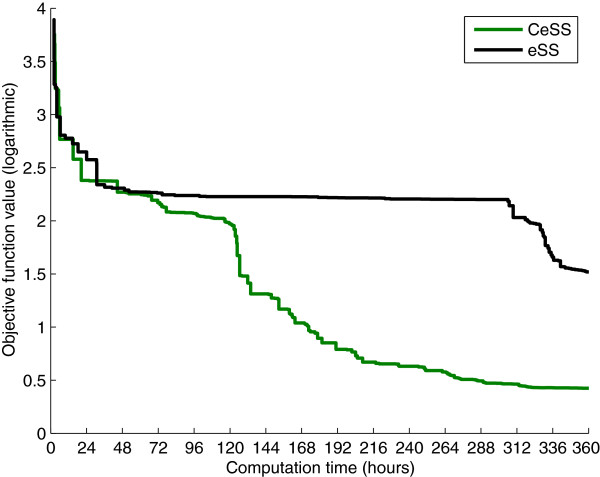
Background: Mathematical models play a key role in systems biology: they summarize the currently available knowledge in a way that allows to make experimentally verifiable predictions. Model calibration consists of finding the parameters that give the best fit to a set of experimental data, which entails minimizing a cost function that measures the goodness of this fit. Most mathematical models in systems biology present three characteristics which make this problem very difficult to solve: they are highly non-linear, they have a large number of parameters to be estimated, and the information content of the available experimental data is frequently scarce. Hence, there is a need for global optimization methods capable of solving this problem efficiently. Results: A new approach for parameter estimation of large scale models, called Cooperative Enhanced Scatter Search (CeSS), is presented. Its key feature is the cooperation between different programs (“threads”) that run in parallel in different processors. Each thread implements a state of the art metaheuristic, the enhanced Scatter Search algorithm (eSS). Cooperation, meaning information sharing between threads, modifies the systemic properties of the algorithm and allows to speed up performance. Two parameter estimation problems involving models related with the central carbon metabolism of E. coli which include different regulatory levels (metabolic and transcriptional) are used as case studies. The performance and capabilities of the method are also evaluated using benchmark problems of large-scale global optimization, with excellent results. Conclusions: The cooperative CeSS strategy is a general purpose technique that can be applied to any model calibration problem. Its capability has been demonstrated by calibrating two large-scale models of different characteristics, improving the performance of previously existing methods in both cases. The cooperative metaheuristic presented here can be easily extended to incorporate other global and local search solvers and specific structural information for particular classes of problems.
Overview
The claims and statistics of this paper haven’t been checked yet.
Free: it reads the open-access text and checks the first 5 claims that cite a source we can check. Create a free account to check every claim.
Integrity signals
Registry
Cites
Statistics
Figures




Verification
Claims the paper makes
The claims and statistics of this paper haven’t been checked yet.
Free: it reads the open-access text and checks the first 5 claims that cite a source we can check. Create a free account to check every claim.
Claims other papers make about this one
Each is checked against this paper’s own text: does it say what the citing paper says it does?
The cited source says what the claim attributes to it.
In the citing paper
“For example, scatter search has proved to be a very efficient method when the local search phase is performed by a specialized local method [114,116].”
From Reverse engineering and identification in systems biology: strategies, perspectives and challenges (2014) · cites this paper as [116]
In the citing paper
“Moreover, they can be parallelized, so their application to large-scale kinetic models is feasible [116].”
From Reverse engineering and identification in systems biology: strategies, perspectives and challenges (2014) · cites this paper as [116]
Self-check
Percentages, sums and reported differences re-computed from the paper’s own numbers.
The self-check needs the paper’s full text.
Citations
Cites
KEGG: Kyoto Encyclopedia of Genes and Genomes
Kanehisa, M. (2000) · Nucleic Acids Research · doi:10.1093/nar/28.1.27 · Cited by 37,077
KEGG: Kyoto Encyclopedia of Genes and Genomes
Ogata, H., Goto, S., Sato, K., Fujibuchi, W., Bono, H., & Kanehisa, M. (1999) · Nucleic Acids Research · doi:10.1093/nar/27.1.29 · Cited by 31,232
Evolution strategies – A comprehensive introduction
Beyer, H.-G., & Schwefel, H.-P. (2002) · Natural Computing · doi:10.1023/a:1015059928466 · Cited by 2,790
Large scale evolutionary optimization using cooperative coevolution
Yang, Z., Tang, K., & Yao, X. (2008) · Information Sciences · doi:10.1016/j.ins.2008.02.017 · Cited by 1,026
LSODE and LSODI, two new initial value ordinary differential equation solvers
Hindmarsh, A. C. (1980) · ACM SIGNUM Newsletter · doi:10.1145/1218052.1218054 · Cited by 907
Integrating high-throughput and computational data elucidates bacterial networks
Covert, M. W., Knight, E. M., Reed, J. L., Herrgard, M. J., & Palsson, B. O. (2004) · Nature · doi:10.1038/nature02456 · Cited by 792
Fundamentals of Scatter Search and Path Relinking
Glover, F., Laguna, M., & Martí, R. (2000) · Cited by 743
Improved evolutionary optimization from genetically adaptive multimethod search
Vrugt, J. A., & Robinson, B. A. (2007) · Proceedings of the National Academy of Sciences · doi:10.1073/pnas.0610471104 · Cited by 614
Chen, W. W., Schoeberl, B., Jasper, P. J., Niepel, M., Nielsen, U. B., Lauffenburger, D. A., & Sorger, P. K. (2009) · Molecular Systems Biology · doi:10.1038/msb.2008.74 · Cited by 391
Systems biology: parameter estimation for biochemical models
Ashyraliyev, M., Fomekong‐Nanfack, Y., Kaandorp, J. A., & Blom, J. G. (2009) · The FEBS Journal · doi:10.1111/j.1742-4658.2008.06844.x · Cited by 323
Research works printed but not linked: 2
- De La Maza M, Yuret D: Dynamic hill climbing. AI EXPERT 1994, 9: 26-26.
- IEEE World Congress on Computational Intelligence (CEC@WCCI-2012): Competition on Large Scale Global Optimization. 2012.http://staff.ustc.edu.cn/~ketang/cec2012/lsgo_competition.htm []
Cited by
Metaheuristics in large-scale global continues optimization: A survey
Mahdavi, S., Shiri, M. E., & Rahnamayan, S. (2015) · Information Sciences · doi:10.1016/j.ins.2014.10.042 · Cited by 465
Penas, D. R., González, P., Egea, J. A., Doallo, R., & Banga, J. R. (2017) · BMC Bioinformatics · doi:10.1186/s12859-016-1452-4 · Cited by 385
Self-citationReverse engineering and identification in systems biology: strategies, perspectives and challenges
Villaverde, A. F., & Banga, J. R. (2014) · Journal of The Royal Society Interface · doi:10.1098/rsif.2013.0505 · Cited by 229
Self-citationEgea, J. A., Henriques, D., Cokelaer, T., Villaverde, A. F., MacNamara, A., Danciu, D.-P., Banga, J. R., & Saez-Rodriguez, J. (2014) · BMC Bioinformatics · doi:10.1186/1471-2105-15-136 · Cited by 176
Self-citationKell, D. B., & Goodacre, R. (2014) · Drug Discovery Today · doi:10.1016/j.drudis.2013.07.014 · Cited by 169
Metadata
- Authors
- Villaverde, A. F., Egea, J. A., & Banga, J. R.
- Affiliations
- Consejo Superior de Investigaciones Científicas (ES)
- Corresponding author
- Banga, Julio R
- Venue
- BMC Systems Biology
- Published
- 2012-06-22
- Volume
- 6
- Issue
- 1
- Pages
- 75-75
- ISSN
- 1752-0509 (ISSN-L)
- PMC
- PMC3512509
- OpenAlex
- W2090517830
- Cited by
- 56
- References
- 38
- Citations by year
- 2024: 4 · 2023: 3 · 2022: 2 · 2021: 1 · 2020: 3 · 2019: 6 · 2018: 6 · 2017: 5 · 2016: 2 · 2015: 11 · 2014: 6 · 2013: 7
- FWCI
- 7.56
- Type
- journal article
- Language
- en
- Open access
- gold
- doi.org
- Licence
- cc-by
- Locations
- BMC Systems Biology (publishedVersion, cc-by)
- PubMed Central (publishedVersion, cc-by)
- PubMed (publishedVersion)
- DIGITAL.CSIC (Spanish National Research Council (CSIC)) (submittedVersion)
- DOAJ (DOAJ: Directory of Open Access Journals) (submittedVersion)
- Funders
- European Commission (289434)
- Ministerio de Economía y Competitividad (DPI2011-28112-C04-04, DPI2011-28112-C04-03, C04-04)
- FP7 Food, Agriculture and Fisheries, Biotechnology
- Topics
- Physical Sciences › Computer Science › Artificial Intelligence › Metaheuristic Optimization Algorithms Research
- Life Sciences › Biochemistry, Genetics and Molecular Biology › Molecular Biology › Gene Regulatory Network Analysis
- Life Sciences › Biochemistry, Genetics and Molecular Biology › Molecular Biology › Microbial Metabolic Engineering and Bioproduction
- Keywords
- parameter estimation, model calibration, systems biology models, cooperative metaheuristics, global optimization, parallel threads, information sharing, central carbon metabolism, Escherichia coli, transcriptional regulation, metabolic regulation, large-scale optimization
- MeSH terms
- Algorithms, Calibration, Carbon, Escherichia coli, Models, Biological, Time Factors, Transcription, Genetic, Gene Expression Regulation, Bacterial, Systems Biology
About these checks
Registry, retraction, Cites and statistics results are computed, not judged, with one exception: a printed reference that no index lists is read once by a model before it counts as a citation error. Claims are extracted by a model and kept only when their quote appears verbatim in the text; each cited source is then checked, with a model’s help, for whether it says what the claim relies on. Those verdicts can be wrong — read the claim’s quote and the cited source before relying on one.
Statistics and arithmetic are recomputed, not judged.
Confidence bands are shown only for fields calibrated on our annotated test set. None is calibrated yet, so no band is shown.
What counts as a claim ›How we measure confidence ›How we check this ›
Are you an author, or do you see a problem with this page? Request a review
How to cite
Cite CoChat for the checks on this page, and the paper for its own findings.
- This page
- CoChat. (2026). Citation check: A cooperative strategy for parameter estimation in large scale systems biology models. https://app.cochat.ai/papers/10.1186/1752-0509-6-75
- The paper
- Villaverde, A. F., Egea, J. A., & Banga, J. R. (2012). A cooperative strategy for parameter estimation in large scale systems biology models. BMC Systems Biology. https://doi.org/10.1186/1752-0509-6-75
Data sources
Bibliographic data: Semantic Scholar, OpenAlex, Crossref.
Contains information from the Semantic Scholar Academic Graph Datasets, made available under the ODC Attribution License (ODC-BY 1.0).
Semantic Scholar’s data is described in: Kinney, R., et al. (2023). The Semantic Scholar Open Data Platform. arXiv:2301.10140.
