

The DOI matches its Crossref record; 84 of the 84 references it cites were found in a registry or an index.
3D deep convolutional neural networks for amino acid environment similarity analysis
Open accessAbstract
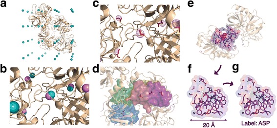
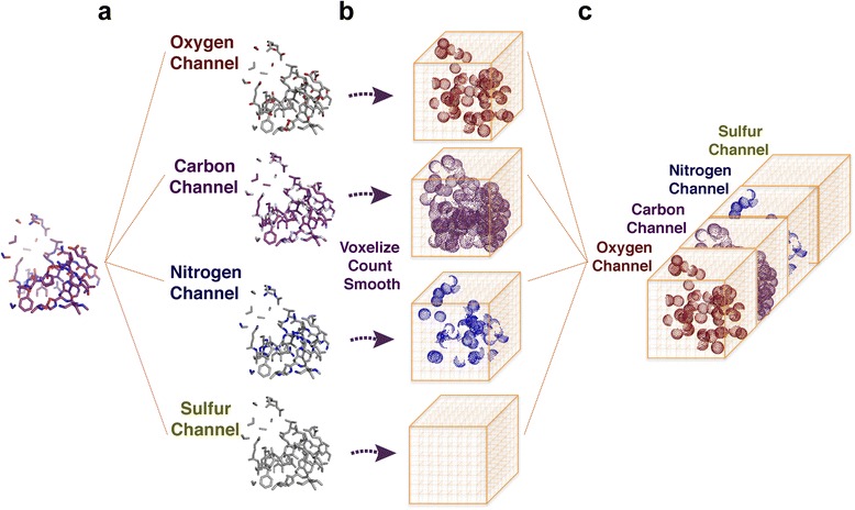
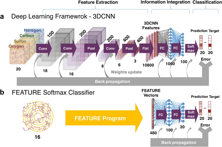
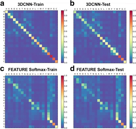
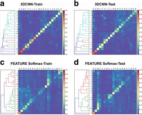
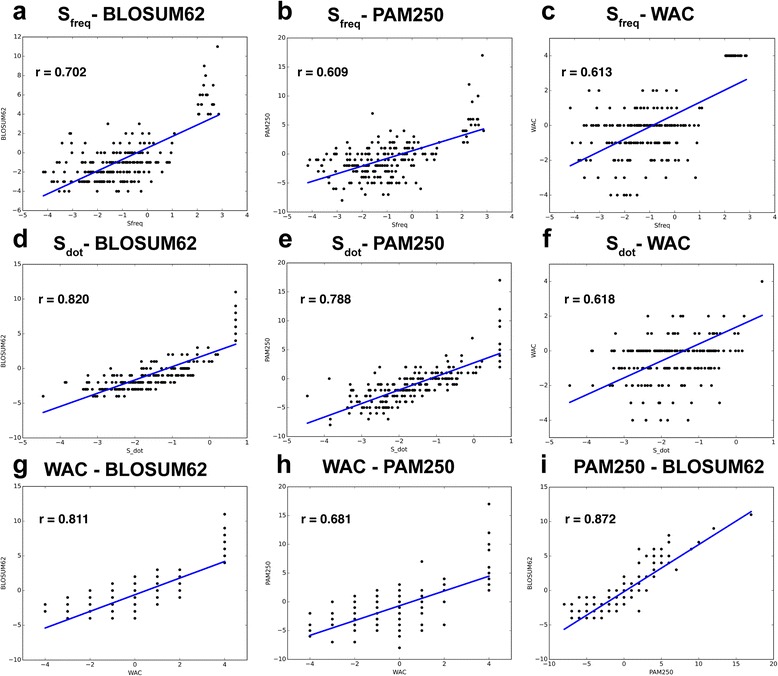
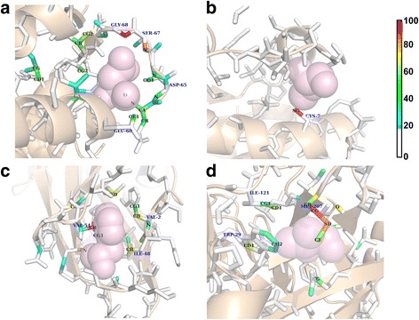
BACKGROUND: Central to protein biology is the understanding of how structural elements give rise to observed function. The surfeit of protein structural data enables development of computational methods to systematically derive rules governing structural-functional relationships. However, performance of these methods depends critically on the choice of protein structural representation. Most current methods rely on features that are manually selected based on knowledge about protein structures. These are often general-purpose but not optimized for the specific application of interest. In this paper, we present a general framework that applies 3D convolutional neural network (3DCNN) technology to structure-based protein analysis. The framework automatically extracts task-specific features from the raw atom distribution, driven by supervised labels. As a pilot study, we use our network to analyze local protein microenvironments surrounding the 20 amino acids, and predict the amino acids most compatible with environments within a protein structure. To further validate the power of our method, we construct two amino acid substitution matrices from the prediction statistics and use them to predict effects of mutations in T4 lysozyme structures. RESULTS: Our deep 3DCNN achieves a two-fold increase in prediction accuracy compared to models that employ conventional hand-engineered features and successfully recapitulates known information about similar and different microenvironments. Models built from our predictions and substitution matrices achieve an 85% accuracy predicting outcomes of the T4 lysozyme mutation variants. Our substitution matrices contain rich information relevant to mutation analysis compared to well-established substitution matrices. Finally, we present a visualization method to inspect the individual contributions of each atom to the classification decisions. CONCLUSIONS: End-to-end trained deep learning networks consistently outperform methods using hand-engineered features, suggesting that the 3DCNN framework is well suited for analysis of protein microenvironments and may be useful for other protein structural analyses.
Overview
The claims and statistics of this paper haven’t been checked yet.
Run the check — free, no account needed. It reads the open-access text and checks the sources it cites.
Integrity signals
Registry
Cites
Statistics
Figures
Verification
Claims the paper makes
The claims and statistics of this paper haven’t been checked yet.
Run the check — free, no account needed. It reads the open-access text and checks the sources it cites.
Claims other papers make about this one
Each is checked against this paper’s own text: does it say what the citing paper says it does?
In the citing paper
“We have previously shown that 3DCNNs can extract meaningful features of amino acid microenvironments directly from raw atom distribution 12 .”
From Graph Convolutional Neural Networks for Predicting Drug-Target Interactions (2019) · cites this paper as [12]
Self-check
Percentages, sums and reported differences re-computed from the paper’s own numbers.
The self-check needs the paper’s full text.
Citations
Cites
ImageNet classification with deep convolutional neural networks
Krizhevsky, A., Sutskever, I., & Hinton, G. E. (2017) · Communications of the ACM · doi:10.1145/3065386 · Cited by 112,155
LeCun, Y., Bengio, Y., & Hinton, G. (2015) · Nature · doi:10.1038/nature14539 · Cited by 84,126
Cortes, C., & Vapnik, V. (1995) · Machine Learning · doi:10.1007/bf00994018 · Cited by 59,421
Regression shrinkage and selection via the lasso
Tibshirani, R. (1996) · Journal of the Royal Statistical Society Series B: Statistical Methodology · doi:10.1111/j.2517-6161.1996.tb02080.x · Cited by 51,482
Going deeper with convolutions
Szegedy, C., Liu, W., Jia, Y., Sermanet, P., Reed, S., Anguelov, D., Erhan, D., Vanhoucke, V., & Rabinovich, A. (2015) · 2015 IEEE Conference on Computer Vision and Pattern Recognition (CVPR) · doi:10.1109/cvpr.2015.7298594 · Cited by 48,562
Berman, H. M. (2000) · Nucleic Acids Research · doi:10.1093/nar/28.1.235 · Cited by 40,196
Cortes, C., & Vapnik, V. N. (1995) · Machine Learning · doi:10.1023/a:1022627411411 · Cited by 34,565
(2014) · Cited by 33,419
Learning representations by back-propagating errors
Rumelhart, D. E., Hinton, G. E., & Williams, R. J. (1986) · Nature · doi:10.1038/323533a0 · Cited by 31,892
Hierarchical Grouping to Optimize an Objective Function
Ward, J. H. (1963) · Journal of the American Statistical Association · doi:10.1080/01621459.1963.10500845 · Cited by 21,341
Research works printed but not linked: 2
- C. M. Bishop, Pattern recognition. 2006.
- B. C. Dayhoff, M.O., Schwartz, R. and Orcutt, “A Model of Evolutionary Change in Proteins,” in Atlas of protein sequence and structure, Volume 5,., National Biomedical Research Foundation Silver Spring, MD, 1978, pp. 345–358
Cited by
Sorted by citations
Machine learning in chemoinformatics and drug discovery
Lo, Y.-C., Rensi, S. E., Torng, W., & Altman, R. B. (2018) · Drug Discovery Today · doi:10.1016/j.drudis.2018.05.010 · Cited by 960
Self-citationTensor field networks: Rotation- and translation-equivariant neural networks for 3D point clouds
Thomas, N., Smidt, T., Kearnes, S., Yang, L., Li, L., Kohlhoff, K., & Riley, P. (2018) · arXiv · doi:10.48550/arxiv.1802.08219 · Cited by 1,303
Graph convolutional networks for computational drug development and discovery
Sun, M., Zhao, S., Gilvary, C. M., Elemento, O., Zhou, J., & Wang, F. (2019) · Briefings in Bioinformatics · doi:10.1093/bib/bbz042 · Cited by 424
Graph Convolutional Neural Networks for Predicting Drug-Target Interactions
Torng, W., & Altman, R. B. (2019) · Journal of Chemical Information and Modeling · doi:10.1021/acs.jcim.9b00628 · Cited by 371
Self-citationArtificial Intelligence for Drug Toxicity and Safety
Basile, A. O., Yahi, A., & Tatonetti, N. P. (2019) · Trends in Pharmacological Sciences · doi:10.1016/j.tips.2019.07.005 · Cited by 401
3D Steerable CNNs: Learning Rotationally Equivariant Features in Volumetric DataPreprint
Weiler, M., Geiger, M., Welling, M., Boomsma, W., & Cohen, T. (2018) · arXiv (Cornell University) · doi:10.48550/arxiv.1807.02547 · Cited by 231
Meller, A., Ward, M. D., Borowsky, J. H., Kshirsagar, M., Lotthammer, J. M., Oviedo, F., Ferres, J. L., & Bowman, G. R. (2023) · Nature Communications · doi:10.1038/s41467-023-36699-3 · Cited by 207
Protein sequence design with a learned potential
Anand, N., Eguchi, R., Mathews, I. I., Perez, C. P., Derry, A., Altman, R. B., & Huang, P.-S. (2022) · Nature Communications · doi:10.1038/s41467-022-28313-9 · Cited by 171
Self-citationInformatics and Computational Methods in Natural Product Drug Discovery: A Review and Perspectives
Romano, J. D., & Tatonetti, N. P. (2019) · Frontiers in Genetics · doi:10.3389/fgene.2019.00368 · Cited by 183
Goshisht, M. K. (2024) · ACS Omega · doi:10.1021/acsomega.3c05913 · Cited by 173
Recent Advances in Machine-Learning-Based Chemoinformatics: A Comprehensive Review
Niazi, S. K., & Mariam, Z. (2023) · International Journal of Molecular Sciences · doi:10.3390/ijms241411488 · Cited by 179
Applications of artificial intelligence to enzyme and pathway design for metabolic engineering
Jang, W. D., Kim, G. B., Kim, Y., & Lee, S. Y. (2021) · Current Opinion in Biotechnology · doi:10.1016/j.copbio.2021.07.024 · Cited by 159
Discovery of Novel Gain-of-Function Mutations Guided by Structure-Based Deep Learning
Shroff, R., Cole, A. W., Diaz, D. J., Morrow, B. R., Donnell, I., Annapareddy, A., Gollihar, J., Ellington, A. D., & Thyer, R. T. (2020) · ACS Synthetic Biology · doi:10.1021/acssynbio.0c00345 · Cited by 144
Li, B., Yang, Y., Capra, J. A., & Gerstein, M. (2020) · PLoS Computational Biology · doi:10.1371/journal.pcbi.1008291 · Cited by 142
Haghighatlari, M., Li, J., Heidar‐Zadeh, F., Liu, Y., Guan, X., & Head-Gordon, T. L. (2020) · Chem · doi:10.1016/j.chempr.2020.05.014 · Cited by 116
Amino acid encoding for deep learning applications
ElAbd, H., Bromberg, Y., Hoarfrost, A., Lenz, T. L., Franke, A., & Wendorff, M. (2020) · BMC Bioinformatics · doi:10.1186/s12859-020-03546-x · Cited by 110
Protein docking model evaluation by 3D deep convolutional neural networks
Wang, X., Terashi, G., Christoffer, C. W., Zhu, M., & Kihara, D. (2019) · Bioinformatics · doi:10.1093/bioinformatics/btz870 · Cited by 105
3D Molecular Representations Based on the Wave Transform for Convolutional Neural Networks
Kuzminykh, D., Polykovskiy, D. A., Kadurin, A., Zhebrak, A., Baskov, I., Nikolenko, S., Shayakhmetov, R., & Zhavoronkov, A. A. (2018) · Molecular Pharmaceutics · doi:10.1021/acs.molpharmaceut.7b01134 · Cited by 107
Deep convolutional networks for quality assessment of protein folds
Derevyanko, G., Grudinin, S., Bengio, Y., & Lamoureux, G. (2018) · Bioinformatics · doi:10.1093/bioinformatics/bty494 · Cited by 103
Casey, A., Son, S. F., Bilionis, I., & Barnes, B. C. (2020) · Journal of Chemical Information and Modeling · doi:10.1021/acs.jcim.0c00259 · Cited by 99
Metal3D: a general deep learning framework for accurate metal ion location prediction in proteins
Dürr, S. L., Levy, A., & Rothlisberger, U. (2023) · Nature Communications · doi:10.1038/s41467-023-37870-6 · Cited by 88
Mathema, V. B., Sen, P., Lamichhane, S., Orešič, M., & Khoomrung, S. (2023) · Computational and Structural Biotechnology Journal · doi:10.1016/j.csbj.2023.01.043 · Cited by 101
Structure-based protein design with deep learning
Ovchinnikov, S., & Huang, P.-S. (2021) · Current Opinion in Chemical Biology · doi:10.1016/j.cbpa.2021.08.004 · Cited by 93
Branda, F., & Scarpa, F. (2024) · Antibiotics · doi:10.3390/antibiotics13060502 · Cited by 104
High precision protein functional site detection using 3D convolutional neural networks
Torng, W., & Altman, R. B. (2019) · Bioinformatics · doi:10.1093/bioinformatics/bty813 · Cited by 69
Self-citationApplication of Machine Learning in Translational Medicine: Current Status and Future Opportunities
Terranova, N., Venkatakrishnan, K., & Benincosa, L. J. (2021) · The AAPS Journal · doi:10.1208/s12248-021-00593-x · Cited by 88
Li, J., Zhu, W., Wang, J., Li, W., Gong, S., Zhang, J., & Wang, W. (2018) · PLoS Computational Biology · doi:10.1371/journal.pcbi.1006514 · Cited by 82
Wilman, W., Wróbel, S., Bielska, W., Deszyński, P., Dudzic, P., Jaszczyszyn, I., Kaniewski, J., Młokosiewicz, J., Rouyan, A., Satława, T., et al. (2022) · Briefings in Bioinformatics · doi:10.1093/bib/bbac267 · Cited by 86
Predicting the pathogenicity of missense variants using features derived from AlphaFold2
Schmidt, A., Röner, S., Mai, K., Klinkhammer, H., Kircher, M., & Ludwig, K. U. (2023) · Bioinformatics · doi:10.1093/bioinformatics/btad280 · Cited by 79
Multiresolution 3D-DenseNet for Chemical Shift Prediction in NMR Crystallography
Liu, S., Li, J., Bennett, K., Ganoe, B., Stauch, T., Head‐Gordon, M., Hexemer, A., Ushizima, D. M., & Head-Gordon, T. L. (2019) · The Journal of Physical Chemistry Letters · doi:10.1021/acs.jpclett.9b01570 · Cited by 72
Rotamer-free protein sequence design based on deep learning and self-consistency
Liu, Y., Zhang, L., Wang, W., Zhu, M., Wang, C., Li, F., Zhang, J., Li, H., Chen, Q., & Liu, H. (2022) · Nature Computational Science · doi:10.1038/s43588-022-00273-6 · Cited by 72
A survey of geometric graph neural networks: data structures, models and applications
Han, J., Cen, J., Wu, L., Li, Z., Kong, X., Jiao, R., Yu, Z., Xu, T., Wu, F., Wang, Z., et al. (2025) · Frontiers of Computer Science · doi:10.1007/s11704-025-41426-w · Cited by 104
Deep learning for mining protein data
Shi, Q., Chen, W., Huang, S., Wang, Y., & Xue, Z. (2019) · Briefings in Bioinformatics · doi:10.1093/bib/bbz156 · Cited by 68
A review on the recent applications of deep learning in predictive drug toxicological studies
Sinha, K., Ghosh, N., & Sil, P. C. (2023) · Chemical Research in Toxicology · doi:10.1021/acs.chemrestox.2c00375 · Cited by 64
Deep Learning for Genomics: From Early Neural Nets to Modern Large Language Models
Yue, T., Wang, Y., Zhang, L., Gu, C., Xue, H., Wang, W., Lyu, Q., & Dun, Y. (2023) · International Journal of Molecular Sciences · doi:10.3390/ijms242115858 · Cited by 192
Improved Bst DNA Polymerase Variants Derived via a Machine Learning Approach
Paik, I., Ngo, P. H. T., Shroff, R., Diaz, D. J., Maranhao, A. C., Walker, D. J. F., Bhadra, S., & Ellington, A. D. (2021) · Biochemistry · doi:10.1021/acs.biochem.1c00451 · Cited by 57
Cortés‐Ciriano, I., & Bender, A. (2019) · Journal of Cheminformatics · doi:10.1186/s13321-019-0364-5 · Cited by 63
Hierarchical, rotation‐equivariant neural networks to select structural models of protein complexes
Eismann, S., Townshend, R. J. L., Thomas, N., Jagota, M., Jing, B., & Dror, R. O. (2020) · Proteins Structure Function and Bioinformatics · doi:10.1002/prot.26033 · Cited by 61
Using machine learning to predict the effects and consequences of mutations in proteins
Diaz, D. J., Kulikova, A. V., Ellington, A. D., & Wilke, C. O. (2023) · Current Opinion in Structural Biology · doi:10.1016/j.sbi.2022.102518 · Cited by 54
DrugAI: a multi-view deep learning model for predicting drug–target activating/inhibiting mechanisms
Zhang, S., Yang, K., Liu, Z., Lai, X., Yang, Z., Zeng, J., & Li, S. (2022) · Briefings in Bioinformatics · doi:10.1093/bib/bbac526 · Cited by 52
Simulations meet machine learning in structural biology
Pérez, A., Martínez-Rosell, G., & Fabritiis, G. D. (2018) · Current Opinion in Structural Biology · doi:10.1016/j.sbi.2018.02.004 · Cited by 51
DLPacker : Deep learning for prediction of amino acid side chain conformations in proteins
Misiura, M., Shroff, R., Thyer, R., & Kolomeisky, A. B. (2022) · Proteins: Structure, Function, and Bioinformatics · doi:10.1002/prot.26311 · Cited by 51
Machine learning accelerates quantum mechanics predictions of molecular crystals
Han, Y., Ali, I., Wang, Z., Cai, J., Wu, S., Tang, J., Zhang, L., Ren, J., Xiao, R., Lu, Q., et al. (2021) · Physics Reports · doi:10.1016/j.physrep.2021.08.002 · Cited by 49
Recent Advances in Machine Learning Variant Effect Prediction Tools for Protein Engineering
Horne, J., & Shukla, D. (2022) · Industrial & Engineering Chemistry Research · doi:10.1021/acs.iecr.1c04943 · Cited by 48
Liu, Q., Wang, P., Zhu, C., Gaines, B. B., Zhu, T., Bi, J., & Song, M. (2021) · Journal of Molecular Graphics and Modelling · doi:10.1016/j.jmgm.2021.107865 · Cited by 46
Bakkers, M. J. G., Ritschel, T., Tiemessen, M. M., Dijkman, J., Zuffianò, A. A., Yu, X., van Overveld, D., Le, L., Voorzaat, R., van Haaren, M. M., et al. (2024) · Nature Communications · doi:10.1038/s41467-024-50659-5 · Cited by 47
Protein Sequence Design with a Learned PotentialPreprint
Anand, N., Eguchi, R. R., Mathews, I. I., Perez, C. P., Derry, A., Altman, R. B., & Huang, P. (2020) · bioRxiv (Cold Spring Harbor Laboratory) · doi:10.1101/2020.01.06.895466 · Cited by 40
Self-citationCortés‐Ciriano, I., & Bender, A. (2019) · Apollo (University of Cambridge) · doi:10.17863/cam.43757 · Cited by 39
Yu, Y., Xu, T., Li, J., Qiu, Y., Rong, Y., Gong, Z., Cheng, X., Dong, L., Liu, W., Li, J., et al. (2021) · ACS Omega · doi:10.1021/acsomega.1c03613 · Cited by 40
ATOM3D: Tasks On Molecules in Three DimensionsPreprint
Townshend, R. J. L., Vögele, M., Suriana, P., Derry, A., Powers, A. S., Laloudakis, Y. D., Balachandar, S., Jing, B., Anderson, B., Eismann, S., et al. (2020) · arXiv (Cornell University) · doi:10.13140/rg.2.2.30339.73765 · Cited by 109
Self-citationProtein representations: Encoding biological information for machine learning in biocatalysis
Harding-Larsen, D., Funk, J., Madsen, N. G., Gharabli, H., Acevedo-Rocha, C. G., Mazurenko, S., & Welner, D. H. (2024) · Biotechnology Advances · doi:10.1016/j.biotechadv.2024.108459 · Cited by 38
Cobdock: an accurate and practical machine learning-based consensus blind docking method
Ugurlu, S. Y., McDonald, D., Lei, H. J., Jones, A. M., Li, S., Tong, H. Y., Butler, M. S., & He, S. (2024) · Journal of Cheminformatics · doi:10.1186/s13321-023-00793-x · Cited by 38
Sato, R., & Ishida, T. (2019) · PLoS ONE · doi:10.1371/journal.pone.0221347 · Cited by 36
Chowdhury, A., Yang, W., Abdelfatah, K. E., Zare, M., Heyden, A., & Terejanu, G. (2020) · Journal of Chemical Theory and Computation · doi:10.1021/acs.jctc.9b00986 · Cited by 31
A Systematic Literature Review of 3D Deep Learning Techniques in Computed Tomography Reconstruction
Rahman, H., Khan, A. R., Sadiq, T., Farooqi, A. H., Khan, I. U., & Lim, W. H. (2023) · Tomography · doi:10.3390/tomography9060169 · Cited by 30
3D Deep Learning on Medical Images: A Review
SINGH, S. P., Wang, L., Gupta, S., Goli, H., Padmanabhan, P., & Gulyás, B. Z. (2020) · Sensors · doi:10.3390/s20185097 · Cited by 60
Kelkar, A., Dallin, B. C., & Lehn, R. C. V. (2020) · The Journal of Physical Chemistry B · doi:10.1021/acs.jpcb.0c05977 · Cited by 27
Machine Learning Based Comparative Analysis of Methods for Enhancer Prediction in Genomic Data
Kaur, A., Chauhan, A. P. S., & Aggarwal, A. K. (2019) · International Conference on Intelligent Communication and Computational Techniques (ICCT) · doi:10.1109/icct46177.2019.8969054 · Cited by 21
Ge, F., Arif, M., & Yu, D. (2021) · Chemometrics and Intelligent Laboratory Systems · doi:10.1016/j.chemolab.2021.104326 · Cited by 21
Artificial Intelligence in Pharmaceutical Field - A Critical Review
Shanbhogue, M. H., Thirumaleshwar, S., Tegginamath, P. K., & Hemanth Kumar, S. (2021) · Current Drug Delivery · doi:10.2174/1567201818666210617100613 · Cited by 21
Assessment and Optimization of Explainable Machine Learning Models Applied to Transcriptomic Data
Zhao, Y., Shao, J., & Asmann, Y. W. (2022) · Genomics Proteomics & Bioinformatics · doi:10.1016/j.gpb.2022.07.003 · Cited by 21
Electron density-based GPT for optimization and suggestion of host–guest binders
Gutiérrez, J. M. P., Granda, J. M., Ayme, J., Bajczyk, M. D., Wilbraham, L., & Cronin, L. (2024) · Nature Computational Science · doi:10.1038/s43588-024-00602-x · Cited by 20
Gaussian representation for image recognition and reinforcement learning of atomistic structure
Christiansen, M.-P. V., Mortensen, H. L., Meldgaard, S. A., & Hammer, B. (2020) · The Journal of Chemical Physics · doi:10.1063/5.0015571 · Cited by 20
TRScore: a 3D RepVGG-based scoring method for ranking protein docking models
Guo, L., He, J., Lin, P., Huang, S., & Wang, J. (2022) · Bioinformatics · doi:10.1093/bioinformatics/btac120 · Cited by 19
Li, B., Luo, S., Wang, W., Xu, J., Liu, D., Shameem, M., Mattila, J., Franklin, M. C., Hawkins, P. G., & Atwal, G. S. (2025) · mAbs · doi:10.1080/19420862.2025.2474521 · Cited by 20
Multi-scale structural analysis of proteins by deep semantic segmentation
Eguchi, R. R., & Huang, P. (2019) · Bioinformatics · doi:10.1093/bioinformatics/btz650 · Cited by 20
Learning the shape of protein microenvironments with a holographic convolutional neural network
Pun, M. N., Ivanov, A., Bellamy, Q., Montague, Z., LaMont, C., Bradley, P. H., Otwinowski, J., & Nourmohammad, A. (2024) · Proceedings of the National Academy of Sciences · doi:10.1073/pnas.2300838121 · Cited by 18
Deep Learning for Protein–Protein Interaction Site Prediction
Jamasb, A. R., Day, B., Cangea, C., Lió, P., & Blundell, T. L. (2021) · Methods in molecular biology · doi:10.1007/978-1-0716-1641-3_16 · Cited by 19
Foundation models of protein sequences: A brief overview
Bjerregaard, A., Groth, P. M., Hauberg, S., Krogh, A., & Boomsma, W. (2025) · Current Opinion in Structural Biology · doi:10.1016/j.sbi.2025.103004 · Cited by 16
(2022) · doi:10.1002/pro.4541 · Cited by 16
Self-citationErtelt, M., Moretti, R., Meiler, J., & Schoeder, C. T. (2025) · Science Advances · doi:10.1126/sciadv.adr7338 · Cited by 15
Artificial Intelligence-Based Drug Design and Discovery
Lo, Y., Ren, G., Honda, H., & Davis, K. L. (2019) · IntechOpen eBooks · doi:10.5772/intechopen.89012 · Cited by 15
Pagès, G., & Grudinin, S. (2018) · arXiv (Cornell University) · Cited by 15
Artificial intelligence driven protein design and sustainable nanomedicine for advanced theranostics
Esmaeilpour, D., Hamblin, M. R., Cheng, J., Khosravi, A., Liu, J., Zarepour, A., Zarrabi, A., Sillanpaa, M., Zare, E. N., Shen, J., et al. (2026) · Bioactive Materials · doi:10.1016/j.bioactmat.2026.01.036 · Cited by 18
A novel three-dimensional deep learning algorithm for classification of power system faults
Srikanth, P., & Koley, C. (2021) · Computers & Electrical Engineering · doi:10.1016/j.compeleceng.2021.107100 · Cited by 14
Understanding structure-guided variant effect predictions using 3D convolutional neural networks
Ramakrishnan, G., Baakman, C. A. B., Heijl, S., Vroling, B., van Horck, R., Hiraki, J., Xue, L. C., & Huynen, M. A. (2023) · Frontiers in Molecular Biosciences · doi:10.3389/fmolb.2023.1204157 · Cited by 14
Kulikova, A. V., Diaz, D. J., Chen, T., Cole, T. J., Ellington, A. D., & Wilke, C. O. (2023) · Scientific Reports · doi:10.1038/s41598-023-40247-w · Cited by 15
Yang, X., Yokokura, S., Nagahama, T., Yamaguchi, M., & Shimada, T. (2022) · Polymers · doi:10.3390/polym14245406 · Cited by 12
OPUS-Mut: Studying the Effect of Protein Mutation through Side-Chain Modeling
Xu, G., Wang, Q., & Ma, J. (2023) · Journal of Chemical Theory and Computation · doi:10.1021/acs.jctc.2c00847 · Cited by 12
Synthetic Biology Meets Machine Learning
Sieow, B. F., Sotto, R. D., Seet, Z. R. D., Hwang, I. Y., & Chang, M. W. (2022) · Methods in molecular biology · doi:10.1007/978-1-0716-2617-7_2 · Cited by 13
Computational protein design with data‐driven approaches: Recent developments and perspectives
Liu, H., & Chen, Q. (2022) · Wiley Interdisciplinary Reviews Computational Molecular Science · doi:10.1002/wcms.1646 · Cited by 13
Guo, L., Qiu, T., & Wang, J. (2023) · IEEE Transactions on NanoBioscience · doi:10.1109/tnb.2023.3274640 · Cited by 11
Wang, G., Zhai, Y.-J., Xue, Z.-Z., & Xu, Y. (2021) · Biomolecules · doi:10.3390/biom11111607 · Cited by 10
Machine Learning Applications in Chemical Kinetics and Thermochemistry
Chen, L.-Y., & Li, Y. (2023) · Challenges and advances in computational chemistry and physics · doi:10.1007/978-3-031-37196-7_7 · Cited by 10
Gupta, A. K., & Raghavachari, K. (2022) · Journal of Chemical Theory and Computation · doi:10.1021/acs.jctc.1c00504 · Cited by 10
Schmidt, C. M., & Smolke, C. D. (2021) · eLife · doi:10.7554/elife.59697 · Cited by 10
DeepInterface: Protein-protein interface validation using 3D Convolutional Neural NetworksPreprint
Balci, A. T., Gümeli, C., Hakouz, A., Yüret, D., Keskin, Ö., & Gürsoy, A. (2019) · bioRxiv (Cold Spring Harbor Laboratory) · doi:10.1101/617506 · Cited by 9
A structure-based deep learning framework for protein engineeringPreprint
Shroff, R., Cole, A. W., Morrow, B. R., Diaz, D. J., Donnell, I., Gollihar, J., Ellington, A. D., & Thyer, R. T. (2019) · bioRxiv (Cold Spring Harbor Laboratory) · doi:10.1101/833905 · Cited by 10
Searching similar local 3D micro-environments in protein structure databases with MicroMiner
Sieg, J., & Rarey, M. (2023) · Briefings in Bioinformatics · doi:10.1093/bib/bbad357 · Cited by 9
Allman, B. E., Vieira, L., Diaz, D. J., & Wilke, C. O. (2025) · Journal of The Royal Society Interface · doi:10.1098/rsif.2024.0598 · Cited by 11
The usage of deep learning algorithm in medical diagnostic of breast cancer
Parikesit, A. A., & Ramanto, K. N. (2019) · Malaysian Journal of Fundamental and Applied Sciences · doi:10.11113/mjfas.v15n2.1231 · Cited by 8
Structure-informed machine learning for drug discovery: a task-centric perspective
Li, Y., Zhan, R.-H., Rao, J., Liu, M., Sang, P., Zeng, X., Zheng, M., Li, X., & Yang, L. (2026) · Briefings in Bioinformatics · doi:10.1093/bib/bbag081 · Cited by 8
Rappoport, D., & Jinich, A. (2023) · Journal of Chemical Information and Modeling · doi:10.1021/acs.jcim.3c00005 · Cited by 9
Silva, J. C. F., Schuster, L. A., Sexson, N., Erdem, M., Hulke, R., Kirst, M., Resende, M. F. R., & Dias, R. (2025) · PLoS Computational Biology · doi:10.1371/journal.pcbi.1013038 · Cited by 8
Hu, Y., Nie, T., Shen, D., & Yu, G. (2018) · IEEE International Conference on Big Data and Smart Computing (BigComp) · doi:10.1109/bigcomp.2018.00018 · Cited by 6
Hierarchical, rotation-equivariant neural networks to predict the structure of protein complexesPreprint
Eismann, S., Townshend, R. J. L., Thomas, N., Jagota, M., Jing, B., & Dror, R. O. (2020) · arXiv (Cornell University) · Cited by 6
Learning the shape of protein micro-environments with a holographic convolutional neural networkPreprint
Pun, M. N., Ivanov, A., Bellamy, Q., Montague, Z., LaMont, C., Bradley, P. H., Otwinowski, J., & Nourmohammad, A. (2022) · bioRxiv (Cold Spring Harbor Laboratory) · doi:10.1101/2022.10.31.514614 · Cited by 7
Xiao, B., Zhang, C., Zhou, J., Wang, S., Meng, H., Wu, M., Zheng, Y., & Yu, R. (2023) · International Journal of Biological Macromolecules · doi:10.1016/j.ijbiomac.2023.125933 · Cited by 5
Big Data analytics for improved prediction of ligand binding and conformational selection
Gupta, S., Baudry, J. Y., & Menon, V. (2023) · Frontiers in Molecular Biosciences · doi:10.3389/fmolb.2022.953984 · Cited by 5
Metadata
- Authors
- Torng, W., & Altman, R. B.
- Affiliations
- Stanford University (US)
- Corresponding author
- Altman, Russ B.
- Venue
- BMC Bioinformatics
- Published
- 2017-06-14
- Volume
- 18
- Issue
- 1
- Pages
- 302-302
- ISSN
- 1471-2105 (ISSN-L)
- PMC
- PMC5472009
- OpenAlex
- W2625768267
- Cited by
- 142
- References
- 82
- Citations by year
- 2026: 6 · 2025: 13 · 2024: 12 · 2023: 23 · 2022: 21 · 2021: 18 · 2020: 15 · 2019: 20 · 2018: 14
- FWCI
- 5.48
- Type
- journal article
- Language
- en
- Open access
- gold
- doi.org
- Locations
- BMC Bioinformatics (publishedVersion, cc-by)
- Europe PMC (PubMed Central) (publishedVersion, other-oa)
- PubMed Central (publishedVersion, cc-by)
- PubMed (publishedVersion)
- DOAJ (DOAJ: Directory of Open Access Journals) (submittedVersion, cc-by-sa)
- Funders
- National Institutes of Health (GM102365, LM05652, HL117798)
- Topics
- Life Sciences › Biochemistry, Genetics and Molecular Biology › Molecular Biology › Protein Structure and Dynamics
- Life Sciences › Biochemistry, Genetics and Molecular Biology › Molecular Biology › Machine Learning in Bioinformatics
- Life Sciences › Pharmacology, Toxicology and Pharmaceutics › Drug Discovery › Computational Drug Discovery Methods
- Keywords
- 3D convolutional neural networks, protein microenvironment, protein structure representation, amino acid substitution matrices, T4 lysozyme, mutation prediction, structure-function relationship, end-to-end deep learning, feature visualization
- MeSH terms
- Amino Acids, Animals, Brain, Nerve Net, ROC Curve, In Situ Hybridization, Area Under Curve, Embryonic Development, Mice, Transcriptome
About these checks
Registry, retraction, Cites and statistics results are computed, not judged, with one exception: a printed reference that no index lists is read once by a model before it counts as a citation error. Claims are extracted by a model and kept only when their quote appears verbatim in the text; each cited source is then checked, with a model’s help, for whether it says what the claim relies on. Those verdicts can be wrong — read the claim’s quote and the cited source before relying on one.
Statistics and arithmetic are recomputed, not judged.
Confidence bands are shown only for fields calibrated on our annotated test set. None is calibrated yet, so no band is shown.
What counts as a claim ›How we measure confidence ›How we check this ›
Are you an author, or do you see a problem with this page? Request a review
