

The DOI matches its Crossref record; 45 of the 45 references it cites were found in a registry or an index.
Dimensionality and Dynamics in the Behavior of C. elegans
Open accessAbstract
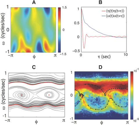
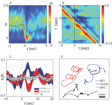
A major challenge in analyzing animal behavior is to discover some underlying simplicity in complex motor actions. Here, we show that the space of shapes adopted by the nematode Caenorhabditis elegans is low dimensional, with just four dimensions accounting for 95% of the shape variance. These dimensions provide a quantitative description of worm behavior, and we partially reconstruct "equations of motion" for the dynamics in this space. These dynamics have multiple attractors, and we find that the worm visits these in a rapid and almost completely deterministic response to weak thermal stimuli. Stimulus-dependent correlations among the different modes suggest that one can generate more reliable behaviors by synchronizing stimuli to the state of the worm in shape space. We confirm this prediction, effectively "steering" the worm in real time.
Overview
The claims and statistics of this paper haven’t been checked yet.
Run the check — free, no account needed. It reads the open-access text and checks the sources it cites.
Integrity signals
Registry
Cites
Statistics
Figures
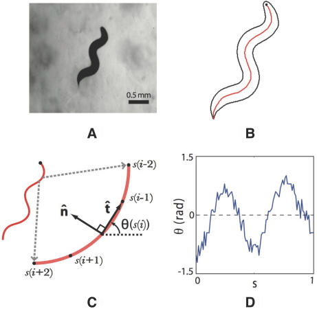
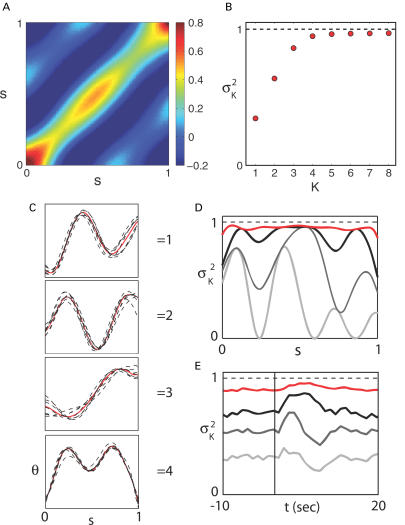
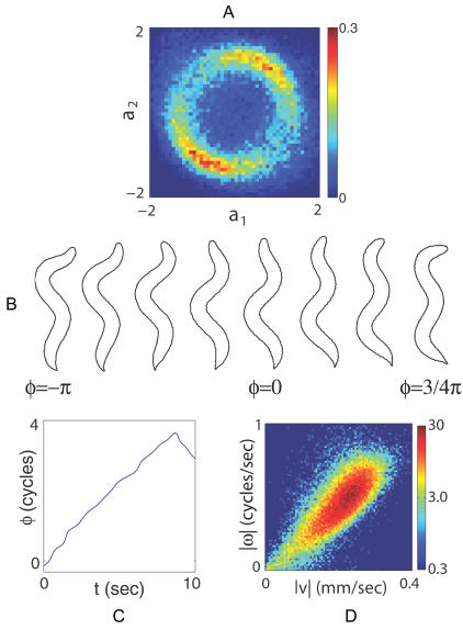
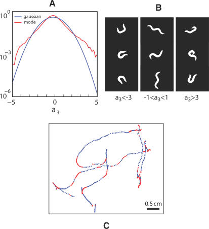
Verification
Claims the paper makes
The claims and statistics of this paper haven’t been checked yet.
Run the check — free, no account needed. It reads the open-access text and checks the sources it cites.
Claims other papers make about this one
Each is checked against this paper’s own text: does it say what the citing paper says it does?
The cited source says what the claim attributes to it.
In the citing paper
“fish larvae require only three basis functions to describe their backbone shapes, whereas worms analyzed in [18] required four.”
From The Behavioral Space of Zebrafish Locomotion and Its Neural Network Analog (2015) · cites this paper as [18]
The cited source says what the claim attributes to it.
In the citing paper
“A study of the invertebrate C. elegans by Stephens et al. [18] provided a powerful method to quantify worm locomotion in terms of the worm’s shapes.”
From The Behavioral Space of Zebrafish Locomotion and Its Neural Network Analog (2015) · cites this paper as [18]
The check wasn’t confident either way, so it gives no verdict — never disputed.
In the citing paper
“However, fish exhibit larger behavioral complexity.”
From The Behavioral Space of Zebrafish Locomotion and Its Neural Network Analog (2015) · cites this paper as [18]
Experimental — accuracy not yet measuredThe check wasn’t confident either way, so it gives no verdict — never disputed.
In the citing paper
“fish are stiffer than worms thanks to their backbone (see Fig 6D), leading to a smaller repertoire of accessible shapes of the fish backbone.”
From The Behavioral Space of Zebrafish Locomotion and Its Neural Network Analog (2015) · cites this paper as [18]
Experimental — accuracy not yet measured
Self-check
Percentages, sums and reported differences re-computed from the paper’s own numbers.
The self-check needs the paper’s full text.
Citations
Cites
THE GENETICS OF CAENORHABDITIS ELEGANS
Brenner, S. (1974) · Genetics · doi:10.1093/genetics/77.1.71 · Cited by 15,161
(1966) · Medical Entomology and Zoology · Cited by 10,293
Signal detection theory and psychophysics
Ingleby, D. (1967) · Journal of Sound and Vibration · doi:10.1016/0022-460x(67)90197-6 · Cited by 8,616
The structure of the nervous system of the nematode Caenorhabditis elegans
White, J. G., Southgate, E., Thomson, J. N., & Brenner, S. (1986) · Philosophical Transactions of the Royal Society of London. B, Biological Sciences · doi:10.1098/rstb.1986.0056 · Cited by 5,589
Genome Sequence of the Nematode C. elegans : A Platform for Investigating Biology
Berg, J. (1998) · Science · doi:10.1126/science.282.5396.2012 · Cited by 4,458
Stochastic Processes in Physics and Chemistry
Cercignani, C. (2005) · Elsevier eBooks · doi:10.1016/b0-12-369401-9/00623-9 · Cited by 2,143
Berg, H. C., & Purcell, E. M. (1977) · Biophysical Journal · doi:10.1016/s0006-3495(77)85544-6 · Cited by 1,758
Lectures on Classical Differential Geometry.
Springer, C. E., & Struik, D. J. (1952) · American Mathematical Monthly · doi:10.2307/2307130 · Cited by 1,370
Postural Hand Synergies for Tool Use
Santello, M., Flanders, M., & Soechting, J. F. (1998) · The Journal of Neuroscience · doi:10.1523/jneurosci.18-23-10105.1998 · Cited by 1,215
The neural and behavioural organization of goal-directed movements
Jeannerod, M. (1988) · Medical Entomology and Zoology · Cited by 1,164
Research works printed but not linked: 1
- J Frenet, 1985, Sur quelque properietès des courbes á double courbure. Thèse, Toulouse, 1847., Abstract in Jour de Math, 17, 437
Cited by
Sorted by citations
Items 501–507 of 507
Better together: Cross and joint covariances enhance signal detectability in undersampled data
Anonymous, Ridout, S. A., & Nemenman, I. M. (2026) · Physical review. E · doi:10.1103/fs5k-y33m
Aging-related behavioral defects in Caenorhabditis elegans
Zeng, J., Chen, C., Iino, Y., & Toyoshima, Y. (2026) · Biology Open · doi:10.1242/bio.062711
Qiu, R., Farkhani, S., Janjua, T. A. M., Canko, E., Pedersen, K., Gastambide, F., Basirat, A., Ebbesen, C. L., & Richter, U. (2026) · bioRxiv (Cold Spring Harbor Laboratory) · doi:10.64898/2026.08.07.743267
The Marginal Value Theorem in Caenorhabditis elegansPreprint
Al‐Asmar, A., Lloret‐Cabot, R., & Pérez‐Escudero, A. (2026) · bioRxiv (Cold Spring Harbor Laboratory) · doi:10.64898/2026.08.10.743854
Kimura, R., & Oku, H. (2026) · IEEE/RAS-EMBS International Conference on Biomedical Robotics and Biomechatronics (BioRob) · doi:10.1109/biorob66782.2026.11681180
Latent factors capturing evolution of behavior in larval zebrafish
Han, C., Gong, Y., Sun, L., Du, J., & Ji, P. (2026) · Chaos An Interdisciplinary Journal of Nonlinear Science · doi:10.1063/5.0354035
A Data-Driven State Machine for Collective Behaviour in C. elegans
Antonic, N., Vellinger, A., & Tuci, E. (2026) · Lecture notes in computer science · doi:10.1007/978-3-032-39953-3_8
Metadata
- Authors
- Stephens, G. J., Johnson-Kerner, B., Bialek, W., & Ryu, W. S.
- Affiliations
- Princeton University (US)
- Corresponding author
- Stephens, Greg J.
- Ryu, William S.
- Venue
- PLoS Computational Biology
- Publisher
- Public Library of Science (PLoS)
- Published
- 2008-04-25
- Volume
- 4
- Issue
- 4
- Pages
- e1000028
- ISSN
- 1553-734X (ISSN-L)
- 1553-7358
- PMC
- PMC2276863
- OpenAlex
- W2142254043
- Cited by
- 509
- References
- 45
- Citations by year
- 2026: 28 · 2025: 28 · 2024: 41 · 2023: 31 · 2022: 38 · 2021: 47 · 2020: 45 · 2019: 48 · 2018: 29 · 2017: 26 · 2016: 22 · 2015: 23 · 2014: 19 · 2013: 19 · 2012: 24
- FWCI
- 5.91
- Type
- journal article
- Language
- en
- Open access
- gold
- doi.org
- Locations
- PLoS Computational Biology (publishedVersion, cc-by)
- PubMed Central (publishedVersion, cc-by)
- PubMed (publishedVersion)
- VU Research Portal (publishedVersion, other-oa)
- arXiv (Cornell University) (submittedVersion)
- RePEc: Research Papers in Economics (submittedVersion)
- DOAJ (DOAJ: Directory of Open Access Journals) (submittedVersion, cc-by-sa)
- Data Archiving and Networked Services (DANS) (submittedVersion, other-oa)
- arXiv (Cornell University)
- Topics
- Life Sciences › Neuroscience › Cellular and Molecular Neuroscience › Neurobiology and Insect Physiology Research
- Physical Sciences › Engineering › Mechanical Engineering › Advanced Materials and Mechanics
- Life Sciences › Neuroscience › Cognitive Neuroscience › Motor Control and Adaptation
- Keywords
- Caenorhabditis elegans, worm locomotion, body shape, equations of motion, attractors, thermal stimuli, behavioral synchronization
- MeSH terms
- Animals, Behavior, Animal, Computer Simulation, Gait, Locomotion, Models, Biological, Caenorhabditis elegans
About these checks
Registry, retraction, Cites and statistics results are computed, not judged, with one exception: a printed reference that no index lists is read once by a model before it counts as a citation error. Claims are extracted by a model and kept only when their quote appears verbatim in the text; each cited source is then checked, with a model’s help, for whether it says what the claim relies on. Those verdicts can be wrong — read the claim’s quote and the cited source before relying on one.
Statistics and arithmetic are recomputed, not judged.
Confidence bands are shown only for fields calibrated on our annotated test set. None is calibrated yet, so no band is shown.
What counts as a claim ›How we measure confidence ›How we check this ›
Are you an author, or do you see a problem with this page? Request a review
