

The DOI matches its Crossref record; 45 of the 46 references it cites were found in a registry or an index; none of the 22 sources its claims cite is checked for support yet.
Comparing Families of Dynamic Causal Models
Open accessAbstract
Mathematical models of scientific data can be formally compared using Bayesian model evidence. Previous applications in the biological sciences have mainly focussed on model selection in which one first selects the model with the highest evidence and then makes inferences based on the parameters of that model. This "best model" approach is very useful but can become brittle if there are a large number of models to compare, and if different subjects use different models. To overcome this shortcoming we propose the combination of two further approaches: (i) family level inference and (ii) Bayesian model averaging within families. Family level inference removes uncertainty about aspects of model structure other than the characteristic of interest. For example: What are the inputs to the system? Is processing serial or parallel? Is it linear or nonlinear? Is it mediated by a single, crucial connection? We apply Bayesian model averaging within families to provide inferences about parameters that are independent of further assumptions about model structure. We illustrate the methods using Dynamic Causal Models of brain imaging data.
Overview
AI snapshot
Written from the paper’s full text.
TL;DR
The paper proposes family-level Bayesian inference and Bayesian model averaging within families as alternatives to selecting a single best model, especially when many models are compared or subjects may use different models. It illustrates the approach with Dynamic Causal Models of fMRI data from an auditory word-processing study, finding evidence that auditory input enters posterior STS and that speech intelligibility modulates forward connections from P to A and P to F.
Key findings
- Family-level inference avoids brittle best-model selection; family posteriors are invariant to the comparison set under fixed effects, and random-effects family inference is implemented via Gibbs sampling.
- For input connectivity, the FFX posterior for region P alone receiving auditory input was 1.00; RFX expected probability was 0.44 with exceedance probability 0.78, while region A alone had RFX exceedance 0.19.
- For modulatory families, the forward family had the highest FFX posterior (0.64) and RFX expected probability (0.52) with exceedance probability 0.66.
- Bayesian model averaging within input family P showed that only forward connections from P to A and P to F were modulated by speech intelligibility; free-energy-based top models averaged 4.5 modulatory connections versus 2.4 in the earlier AIC/BIC-based study.
Methods
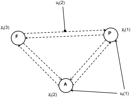
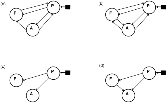
- Dynamic Causal Models for fMRI were used with three regions: left posterior superior temporal sulcus (P), left anterior superior temporal sulcus (A), and pars orbitalis of the inferior frontal gyrus (F); all models had all-to-all endogenous connectivity, with variation in direct input regions and modulatory connections.
- The model space crossed 64 modulatory patterns with 7 input patterns, giving 448 DCMs, fitted to data from a previously published intelligible-speech study; the subject count is not recoverable from the provided text.
- Analysis used fixed-effects and random-effects family-level inference; RFX inference used Gibbs sampling with 10,000 discarded burn-in samples, and Bayesian model averaging was performed within families using Occam’s window.
Limitations
- Stated: the variational Bayes implementation is not accurate for small prior counts, motivating Gibbs sampling; Gibbs sampling is preferred when the number of models exceeds the number of subjects, while VB is preferred for small model sets.
- Stated: the relative merits of different model-evidence criteria are left to a future publication, and the automatic relevance determination approach for DCMs is currently hypothetical.
- Evident from the text: the method is illustrated on one fMRI dataset from an auditory word-processing study, so broader biological applicability is proposed but not tested here; results also depend on the chosen family partitions and on the free-energy approximation to model evidence.
Model-written summary. Check it against the paper before relying on it.
Integrity signals
Registry
Cites
Statistics
Figures
Verification
Claims the paper makes
33 Own interpretation · 20 Not checked yet · 13 Own result · 6 No basis given
The paper states this without a source or data behind it here, so there is nothing to check it against. The quote shows it is in the paper.
In the paper
“However, for group random effects inference the ranking of models can be critically dependent on the comparison set.”
§ Comparing Families of Dynamic Causal Models > Materials and Methods > Comparison Set
plaincorrelational- Asserted: passes — The authors put it forward as true.
- Checkable: passes — It can be checked against evidence.
- Load-bearing: passes — The paper’s conclusions depend on it.
- Based: passes — The paper gives a reason why it holds.
The paper states this without a source or data behind it here, so there is nothing to check it against. The quote shows it is in the paper.
In the paper
“For FFX analysis the relative ranking of a pair of models is not dependent on .”
§ Comparing Families of Dynamic Causal Models > Materials and Methods > Comparison Set
plain- Asserted: passes — The authors put it forward as true.
- Checkable: passes — It can be checked against evidence.
- Load-bearing: unclear — It is unclear whether the paper’s conclusions depend on it.
- Based: passes — The paper gives a reason why it holds.
The paper states this without a source or data behind it here, so there is nothing to check it against. The quote shows it is in the paper.
In the paper
“Second, we emphasise that posterior model probabilities depend on the comparison set.”
§ Comparing Families of Dynamic Causal Models > Materials and Methods > Comparison Set
plaindirect- Asserted: passes — The authors put it forward as true.
- Checkable: passes — It can be checked against evidence.
- Load-bearing: passes — The paper’s conclusions depend on it.
- Based: passes — The paper gives a reason why it holds.
The paper states this without a source or data behind it here, so there is nothing to check it against. The quote shows it is in the paper.
In the paper
“In random effects analysis, augmenting the comparison set with a single extra model can, for example, reverse the ranking of the best and second best models.”
§ Comparing Families of Dynamic Causal Models > Introduction
plaindirect- Asserted: passes — The authors put it forward as true.
- Checkable: passes — It can be checked against evidence.
- Load-bearing: passes — The paper’s conclusions depend on it.
- Based: unclear — It is unclear why the paper says it holds.
A result the paper reports from its own data — it cites no other source for it, so there is none to check. The quote shows it is in the paper.
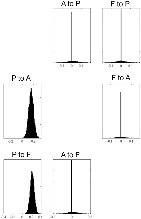
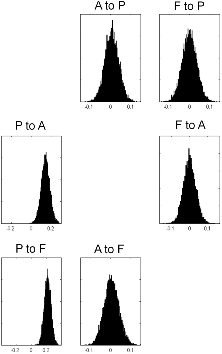
In the paper
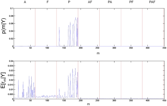
“Both the RFX and FFX model averages within family P show that only connections from P to A, and from P to F, are facilitated by speech intelligibility.”
§ Comparing Families of Dynamic Causal Models > Results > Model Averaging
plaindirect- Asserted: passes — The authors put it forward as true.
- Checkable: passes — It can be checked against evidence.
- Load-bearing: passes — The paper’s conclusions depend on it.
- Based: passes — The paper gives a reason why it holds.
- The authors state this as an assumption: Under the fixed-effects (FFX) assumption, all subjects use the same model.
- The authors state this as an assumption: Under the random-effects (RFX) assumption, each subject uses their own model.
In the paper
“This is exactly the winning model from earlier work [17] (based on AIC/BIC approximation of model evidence).”
§ Comparing Families of Dynamic Causal Models > Discussion
What the sources say
- Not checked yetcites [17] A Leff, 2008, The cortical dynamics of intelligible speech., J Neurosci source
plain- Asserted: passes — The authors put it forward as true.
- Checkable: passes — It can be checked against evidence.
- Load-bearing: unclear — It is unclear whether the paper’s conclusions depend on it.
- Based: passes — The paper gives a reason why it holds.
A result the paper reports from its own data — it cites no other source for it, so there is none to check. The quote shows it is in the paper.
In the paper
“Interestingly, the use of BMA produced an average network structure with speech input to region P, and modulatory connections from P to A and from P to F.”
§ Comparing Families of Dynamic Causal Models > Discussion
plaindirect- Asserted: passes — The authors put it forward as true.
- Checkable: passes — It can be checked against evidence.
- Load-bearing: unclear — It is unclear whether the paper’s conclusions depend on it.
- Based: passes — The paper gives a reason why it holds.
A result the paper reports from its own data — it cites no other source for it, so there is none to check. The quote shows it is in the paper.
In the paper
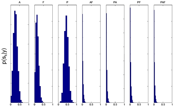
“But we can say, with high confidence (total exceedance probability, ) that either region A alone or region P alone receives auditory input.”
§ Comparing Families of Dynamic Causal Models > Results > Input Regions
boosted- Asserted: passes — The authors put it forward as true.
- Checkable: passes — It can be checked against evidence.
- Load-bearing: passes — The paper’s conclusions depend on it.
- Based: passes — The paper gives a reason why it holds.
- The authors state this as an assumption: Under the random-effects (RFX) assumption, each subject uses their own model.
The paper states this without a source or data behind it here, so there is nothing to check it against. The quote shows it is in the paper.
In the paper
“This model has input to region P and modulatory connections as shown in Figure 6(a).”
§ Comparing Families of Dynamic Causal Models > Results > Relating Family and Model Levels
plain- Asserted: passes — The authors put it forward as true.
- Checkable: passes — It can be checked against evidence.
- Load-bearing: unclear — It is unclear whether the paper’s conclusions depend on it.
- Based: passes — The paper gives a reason why it holds.
- The authors state this as an assumption: Under the fixed-effects (FFX) assumption, all subjects use the same model.
A result the paper reports from its own data — it cites no other source for it, so there is none to check. The quote shows it is in the paper.
In the paper
“The maximum posterior model for the input family inference is model number 185 having posterior probability .”
§ Comparing Families of Dynamic Causal Models > Results > Relating Family and Model Levels
plain- Asserted: passes — The authors put it forward as true.
- Checkable: passes — It can be checked against evidence.
- Load-bearing: unclear — It is unclear whether the paper’s conclusions depend on it.
- Based: passes — The paper gives a reason why it holds.
- The authors state this as an assumption: Under the fixed-effects (FFX) assumption, all subjects use the same model.
In the paper
“One notable difference arising from this distinction is that the top-ranked models in [17] contained significantly fewer connections than those in this paper (one sample t-test, ). The top 10 models in [17] contained an average 2.4 modulatory connections whereas those in this paper contained an average of 4.5.”
§ Comparing Families of Dynamic Causal Models > Results > Relating Family and Model Levels
What the sources say
- Not checked yetcites [17] A Leff, 2008, The cortical dynamics of intelligible speech., J Neurosci source
plaincorrelational- Asserted: passes — The authors put it forward as true.
- Checkable: passes — It can be checked against evidence.
- Load-bearing: passes — The paper’s conclusions depend on it.
- Based: passes — The paper gives a reason why it holds.
In the paper
“The model evidence for the DCMs fitted in this paper was computed using the free energy approximation whereas previous work used (the most conservative of) AIC and BIC [17]. This resulted in the highly ranked models containing significantly more connections than in the previous study.”
§ Comparing Families of Dynamic Causal Models > Discussion
What the sources say
- Not checked yetcites [17] A Leff, 2008, The cortical dynamics of intelligible speech., J Neurosci source
plaindirect- Asserted: passes — The authors put it forward as true.
- Checkable: passes — It can be checked against evidence.
- Load-bearing: passes — The paper’s conclusions depend on it.
- Based: passes — The paper gives a reason why it holds.
A result the paper reports from its own data — it cites no other source for it, so there is none to check. The quote shows it is in the paper.
In the paper
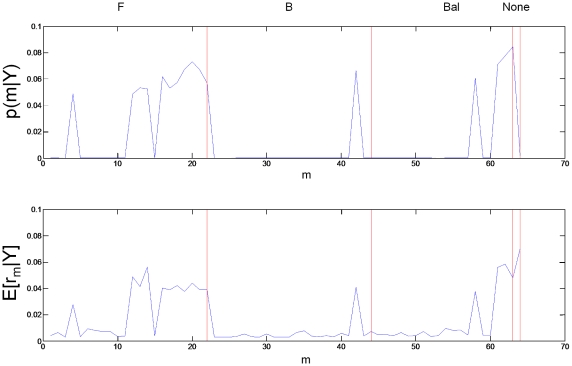
“The first two numerical columns of Table 1 show the posterior family probabilities from an FFX analysis computed using equation 21. These are overwhelmingly in support of models in which region P alone receives auditory input (alternative probability ).”
§ Comparing Families of Dynamic Causal Models > Results > Input Regions
boosted- Asserted: passes — The authors put it forward as true.
- Checkable: passes — It can be checked against evidence.
- Load-bearing: passes — The paper’s conclusions depend on it.
- Based: passes — The paper gives a reason why it holds.
- The authors state this as an assumption: Under the fixed-effects (FFX) assumption, all subjects use the same model.
A result the paper reports from its own data — it cites no other source for it, so there is none to check. The quote shows it is in the paper.
In the paper
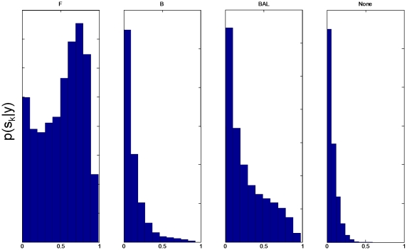
“The conclusions we draw, in this case, are identical to those from the FFX analysis.”
§ Comparing Families of Dynamic Causal Models > Results > Forward versus Backward
plain- Asserted: passes — The authors put it forward as true.
- Checkable: passes — It can be checked against evidence.
- Load-bearing: unclear — It is unclear whether the paper’s conclusions depend on it.
- Based: passes — The paper gives a reason why it holds.
- The authors state this as an assumption: Under the random-effects (RFX) assumption, each subject uses their own model.
A result the paper reports from its own data — it cites no other source for it, so there is none to check. The quote shows it is in the paper.
In the paper
“It is not, however, the best model as indicated by the free energy.”
§ Comparing Families of Dynamic Causal Models > Discussion
plain- Asserted: passes — The authors put it forward as true.
- Checkable: passes — It can be checked against evidence.
- Load-bearing: unclear — It is unclear whether the paper’s conclusions depend on it.
- Based: passes — The paper gives a reason why it holds.
In the paper
“Previous applications in the biological sciences have mainly focussed on model selection in which one first selects the model with the highest evidence and then makes inferences based on the parameters of that model.”
- Also stated in: § Introduction · plain
“Much previous practice in these areas has focussed on model selection in which one first selects the model with the highest evidence and then makes inferences based on the parameters of that model [15]–[18].”
§ Comparing Families of Dynamic Causal Models > Abstract
What the sources say
- Not checked yetcites [15]–[18]
plain- Asserted: passes — The authors put it forward as true.
- Checkable: passes — It can be checked against evidence.
- Load-bearing: passes — The paper’s conclusions depend on it.
- Based: passes — The paper gives a reason why it holds.
- Also stated in: § Introduction · plain
A conclusion the paper draws from its own results — it cites no other source for it, so there is none to check. The quote shows it is in the paper.
In the paper
“We apply Bayesian model averaging within families to provide inferences about parameters that are independent of further assumptions about model structure.”
§ Comparing Families of Dynamic Causal Models > Abstract
plain- Asserted: passes — The authors put it forward as true.
- Checkable: passes — It can be checked against evidence.
- Load-bearing: passes — The paper’s conclusions depend on it.
- Based: unclear — It is unclear why the paper says it holds.
A conclusion the paper draws from its own results — it cites no other source for it, so there is none to check. The quote shows it is in the paper.
In the paper
“This brittleness, refers to the fact that which is the best model can depend critically on which set of models are being compared.”
§ Comparing Families of Dynamic Causal Models > Introduction
plainconditional- Asserted: passes — The authors put it forward as true.
- Checkable: passes — It can be checked against evidence.
- Load-bearing: passes — The paper’s conclusions depend on it.
- Based: passes — The paper gives a reason why it holds.
In the paper
“Family level inference addresses the issue of ‘dilution’ in model selection [4].”
§ Comparing Families of Dynamic Causal Models > Materials and Methods > Family Inference
What the sources say
- Not checked yetcites [4] J Hoeting, 1999, Bayesian Model Averaging: A Tutorial., Statistical Science
plaindirect- Asserted: passes — The authors put it forward as true.
- Checkable: passes — It can be checked against evidence.
- Load-bearing: passes — The paper’s conclusions depend on it.
- Based: passes — The paper gives a reason why it holds.
A conclusion the paper draws from its own results — it cites no other source for it, so there is none to check. The quote shows it is in the paper.
In the paper
“If, for example, a parameter is unchanged from its prior, there will be no penalty.”
§ Comparing Families of Dynamic Causal Models > Materials and Methods > Model Evidence
plain- Asserted: passes — The authors put it forward as true.
- Checkable: passes — It can be checked against evidence.
- Load-bearing: passes — The paper’s conclusions depend on it.
- Based: passes — The paper gives a reason why it holds.
In the paper
“The robustness and accuracy of this method was verified via simulations using data from synthetic populations with known frequencies of competing models [19].”
§ Comparing Families of Dynamic Causal Models > Materials and Methods > Random Effects Analysis
What the sources say
- Not checked yetcites [19] K Stephan, 2009, Bayesian model selection for group studies., Neuroimage source
plain- Asserted: passes — The authors put it forward as true.
- Checkable: passes — It can be checked against evidence.
- Load-bearing: passes — The paper’s conclusions depend on it.
- Based: passes — The paper gives a reason why it holds.
A conclusion the paper draws from its own results — it cites no other source for it, so there is none to check. The quote shows it is in the paper.
In the paper
“This difference reflects the fact that the AIC/BIC approximation to the log evidence penalizes models for each additional connection (parameter) without considering interdependencies or covariances amongst parameters, whereas the free energy approximation takes such dependencies into account.”
§ Comparing Families of Dynamic Causal Models > Results > Relating Family and Model Levels
plaindirect- Asserted: passes — The authors put it forward as true.
- Checkable: passes — It can be checked against evidence.
- Load-bearing: passes — The paper’s conclusions depend on it.
- Based: passes — The paper gives a reason why it holds.
A conclusion the paper draws from its own results — it cites no other source for it, so there is none to check. The quote shows it is in the paper.
In the paper
“Bayesian model averaging can then be used to provide a summary measure of likely parameter values for each family.”
§ Comparing Families of Dynamic Causal Models > Discussion
plain- Asserted: passes — The authors put it forward as true.
- Checkable: passes — It can be checked against evidence.
- Load-bearing: passes — The paper’s conclusions depend on it.
- Based: passes — The paper gives a reason why it holds.
A conclusion the paper draws from its own results — it cites no other source for it, so there is none to check. The quote shows it is in the paper.
In the paper
“For the applications in this paper, the posterior densities from equation 27 will therefore correspond to a mixture of delta functions and Gaussians because for DCMs have a Gaussian form.”
§ Comparing Families of Dynamic Causal Models > Materials and Methods > Bayesian Model Averaging
plaindirect- Asserted: passes — The authors put it forward as true.
- Checkable: passes — It can be checked against evidence.
- Load-bearing: unclear — It is unclear whether the paper’s conclusions depend on it.
- Based: passes — The paper gives a reason why it holds.
- Rests on an assumption: Dynamic causal models (DCMs) have a Gaussian form.
In the paper
“Additionally, the use of Gibbs sampling allows us to relax the assumption made in VB that the posterior densities over and factorise [19].”
§ Comparing Families of Dynamic Causal Models > Materials and Methods > Random Effects Analysis
What the sources say
- Not checked yetcites [19] K Stephan, 2009, Bayesian model selection for group studies., Neuroimage source
plaindirect- Asserted: passes — The authors put it forward as true.
- Checkable: passes — It can be checked against evidence.
- Load-bearing: passes — The paper’s conclusions depend on it.
- Based: passes — The paper gives a reason why it holds.
A conclusion the paper draws from its own results — it cites no other source for it, so there is none to check. The quote shows it is in the paper.
In the paper
“This is due to a bias in the AIC/BIC criterion which leads to overly simple models being selected.”
§ Comparing Families of Dynamic Causal Models > Discussion
plaindirect- Asserted: passes — The authors put it forward as true.
- Checkable: passes — It can be checked against evidence.
- Load-bearing: passes — The paper’s conclusions depend on it.
- Based: passes — The paper gives a reason why it holds.
A conclusion the paper draws from its own results — it cites no other source for it, so there is none to check. The quote shows it is in the paper.
In the paper
“One can see from equation 27 that models with low probability contribute little to the estimate of the marginal density.”
§ Comparing Families of Dynamic Causal Models > Materials and Methods > Bayesian Model Averaging
plaindirect- Asserted: passes — The authors put it forward as true.
- Checkable: passes — It can be checked against evidence.
- Load-bearing: unclear — It is unclear whether the paper’s conclusions depend on it.
- Based: passes — The paper gives a reason why it holds.
None of the sources cited for this claim have been checked yet.
In the paper
“This adaptability makes the Free Energy a better approximation to the model evidence, as has been shown empirically [6],[31].”
§ Comparing Families of Dynamic Causal Models > Materials and Methods > Model Evidence
What the sources say
- Not checked yetcites [6] M Beal, 2003, The Variational Bayesian EM algorithms for incomplete data: with application to scoring graphical model structures. source
- Not checked yetcites [31] S Roberts, 2002, Variational Bayes for Generalised Autoregressive models., IEEE Transactions on Signal Processing source
boosteddirect- Asserted: passes — The authors put it forward as true.
- Checkable: passes — It can be checked against evidence.
- Load-bearing: passes — The paper’s conclusions depend on it.
- Based: passes — The paper gives a reason why it holds.
A conclusion the paper draws from its own results — it cites no other source for it, so there is none to check. The quote shows it is in the paper.
In the paper
“A uniform prior over family probabilities can be obtained by setting for all .”
§ Comparing Families of Dynamic Causal Models > Materials and Methods > Family Inference
plaindirect- Asserted: passes — The authors put it forward as true.
- Checkable: passes — It can be checked against evidence.
- Load-bearing: passes — The paper’s conclusions depend on it.
- Based: passes — The paper gives a reason why it holds.
A conclusion the paper draws from its own results — it cites no other source for it, so there is none to check. The quote shows it is in the paper.
In the paper
“The posterior densities from equation 27 will therefore include a delta function at zero, the height of which corresponds to the posterior probability mass of models which assume that the parameter is zero.”
§ Comparing Families of Dynamic Causal Models > Materials and Methods > Bayesian Model Averaging
plaincorrelational- Asserted: passes — The authors put it forward as true.
- Checkable: passes — It can be checked against evidence.
- Load-bearing: passes — The paper’s conclusions depend on it.
- Based: passes — The paper gives a reason why it holds.
A conclusion the paper draws from its own results — it cites no other source for it, so there is none to check. The quote shows it is in the paper.
In the paper
“Grouping models into families, and setting model priors according to eg. equation 24, achieves exactly this.”
§ Comparing Families of Dynamic Causal Models > Materials and Methods > Family Inference
boosteddirect- Asserted: passes — The authors put it forward as true.
- Checkable: passes — It can be checked against evidence.
- Load-bearing: passes — The paper’s conclusions depend on it.
- Based: passes — The paper gives a reason why it holds.
In the paper
“One way of avoiding this problem is to use priors which dilute the probability within subsets of similar models ([4]).”
§ Comparing Families of Dynamic Causal Models > Materials and Methods > Family Inference
What the sources say
- Not checked yetcites [4] J Hoeting, 1999, Bayesian Model Averaging: A Tutorial., Statistical Science
plaindirect- Asserted: passes — The authors put it forward as true.
- Checkable: passes — It can be checked against evidence.
- Load-bearing: passes — The paper’s conclusions depend on it.
- Based: passes — The paper gives a reason why it holds.
In the paper
“If one uses uniform model priors and many models are similar, then excessive prior probability is allocated to this set of similar models.”
§ Comparing Families of Dynamic Causal Models > Materials and Methods > Family Inference
What the sources say
- Not checked yetcites [4] J Hoeting, 1999, Bayesian Model Averaging: A Tutorial., Statistical Science
plaindirect- Asserted: passes — The authors put it forward as true.
- Checkable: passes — It can be checked against evidence.
- Load-bearing: passes — The paper’s conclusions depend on it.
- Based: passes — The paper gives a reason why it holds.
In the paper
“Reassuringly, posterior confidence regions found using the nonlinear variational approach have been found to be very similar to those obtained using a computationally more expensive sample-based algorithm [26].”
§ Comparing Families of Dynamic Causal Models > Materials and Methods > Dynamic Causal Models
What the sources say
- Not checked yetcites [26] J Chumbley, 2007, A Metropolis-Hastings algorithm for dynamic causal models., Neuroimage source
boosted- Asserted: passes — The authors put it forward as true.
- Checkable: passes — It can be checked against evidence.
- Load-bearing: unclear — It is unclear whether the paper’s conclusions depend on it.
- Based: passes — The paper gives a reason why it holds.
A conclusion the paper draws from its own results — it cites no other source for it, so there is none to check. The quote shows it is in the paper.
In the paper
“We stress that no additional assumptions are required to implement equation 27.”
§ Comparing Families of Dynamic Causal Models > Materials and Methods > Bayesian Model Averaging
plain- Asserted: passes — The authors put it forward as true.
- Checkable: passes — It can be checked against evidence.
- Load-bearing: unclear — It is unclear whether the paper’s conclusions depend on it.
- Based: passes — The paper gives a reason why it holds.
A conclusion the paper draws from its own results — it cites no other source for it, so there is none to check. The quote shows it is in the paper.
In the paper
“Although it is fairly simple to compute the MAP estimates of the Bayesian parameter (MAP) averages analytically, the full posteriors per se have a complicated form. This is because they are mixtures of Gaussians (and delta functions for models where some parameters are precluded a priori).”
§ Comparing Families of Dynamic Causal Models > Materials and Methods > Bayesian Model Averaging
plaindirect- Asserted: passes — The authors put it forward as true.
- Checkable: passes — It can be checked against evidence.
- Load-bearing: unclear — It is unclear whether the paper’s conclusions depend on it.
- Based: passes — The paper gives a reason why it holds.
In the paper
“The ARD approach provides an estimate of the marginal density directly without recourse to Bayesian model averaging.”
§ Comparing Families of Dynamic Causal Models > Discussion
What the sources say
- Not checked yetcites [41] DJC MacKay, 1993, Bayesian non-linear modeling for the prediction competition.
plaindirect- Asserted: passes — The authors put it forward as true.
- Checkable: passes — It can be checked against evidence.
- Load-bearing: unclear — It is unclear whether the paper’s conclusions depend on it.
- Based: passes — The paper gives a reason why it holds.
A conclusion the paper draws from its own results — it cites no other source for it, so there is none to check. The quote shows it is in the paper.
In the paper
“The Discrete approach allows for quantitative family-level inferences about issues such as whether processing is serial or parallel, linear or nonlinear.”
§ Comparing Families of Dynamic Causal Models > Discussion
plaindirect- Asserted: passes — The authors put it forward as true.
- Checkable: passes — It can be checked against evidence.
- Load-bearing: passes — The paper’s conclusions depend on it.
- Based: passes — The paper gives a reason why it holds.
- Probably not a substantial claim. 15
- It may state two separate claims as one. 22
- The quote only partly states this claim. 4
The paper states this without a source or data behind it here, so there is nothing to check it against. The quote shows it is in the paper.
In the paper
“Figure 7 shows the posterior densities of average modulatory connections (averaging over models and subjects). The height of the delta functions in these histograms correspond to the total posterior probability mass of models which assume that the connection is zero.”
§ Comparing Families of Dynamic Causal Models > Results > Model Averaging
plain- Asserted: passes — The authors put it forward as true.
- Checkable: passes — It can be checked against evidence.
- Load-bearing: fails — The paper’s conclusions may not depend on it.
- Based: passes — The paper gives a reason why it holds.
Probably not a substantial claim. The paper’s conclusions may not depend on it. It may state two separate claims as one.
- The authors state this as an assumption: Under the fixed-effects (FFX) assumption, all subjects use the same model.
A result the paper reports from its own data — it cites no other source for it, so there is none to check. The quote shows it is in the paper.
In the paper
“The worst one is with . The posterior odds of the best relative to the worst is only (the largest it could be is ), meaning these models are not significantly better than one another.”
§ Comparing Families of Dynamic Causal Models > Results > Model Averaging
plain- Asserted: passes — The authors put it forward as true.
- Checkable: passes — It can be checked against evidence.
- Load-bearing: passes — The paper’s conclusions depend on it.
- Based: passes — The paper gives a reason why it holds.
It may state two separate claims as one.
- The authors state this as an assumption: Under the fixed-effects (FFX) assumption, all subjects use the same model.
A result the paper reports from its own data — it cites no other source for it, so there is none to check. The quote shows it is in the paper.
In the paper
“Out of these two possibilities it is much more likely that region P alone receives auditory input (exceedance probability ) rather than region A (exceedance probability ).”
§ Comparing Families of Dynamic Causal Models > Results > Input Regions
hedged- Asserted: passes — The authors put it forward as true.
- Checkable: passes — It can be checked against evidence.
- Load-bearing: passes — The paper’s conclusions depend on it.
- Based: passes — The paper gives a reason why it holds.
It may state two separate claims as one. The quote only partly states this claim.
- The authors state this as an assumption: Under the random-effects (RFX) assumption, each subject uses their own model.
In the paper
“It turns out that although the variational algorithm is robust for , it is not accurate for .”
§ Comparing Families of Dynamic Causal Models > Materials and Methods > Random Effects Analysis
What the sources say
- Not checked yetcites Text S1
plain- Asserted: passes — The authors put it forward as true.
- Checkable: passes — It can be checked against evidence.
- Load-bearing: passes — The paper’s conclusions depend on it.
- Based: passes — The paper gives a reason why it holds.
It may state two separate claims as one.
A result the paper reports from its own data — it cites no other source for it, so there is none to check. The quote shows it is in the paper.
In the paper
“For RFX inference the input was inferred to most likely enter region P alone (posterior exceedance probability, ). In the RFX model averaging the Occam's windowing procedure was specific to each subject, thus each subject can have a different number of models in Occam's window. For the input model P family there were an average of models in Occam's window and Figure 8 shows the posterior densities”
§ Comparing Families of Dynamic Causal Models > Results > Model Averaging
plain- Asserted: passes — The authors put it forward as true.
- Checkable: passes — It can be checked against evidence.
- Load-bearing: unclear — It is unclear whether the paper’s conclusions depend on it.
- Based: passes — The paper gives a reason why it holds.
It may state two separate claims as one. The quote only partly states this claim.
- The authors state this as an assumption: Under the random-effects (RFX) assumption, each subject uses their own model.
A result the paper reports from its own data — it cites no other source for it, so there is none to check. The quote shows it is in the paper.
In the paper
“| Forward, | 0.64 | −0.44 | 0.52 | 0.66 |”
§ Comparing Families of Dynamic Causal Models > Results > Forward versus Backward
plain- Asserted: passes — The authors put it forward as true.
- Checkable: passes — It can be checked against evidence.
- Load-bearing: passes — The paper’s conclusions depend on it.
- Based: passes — The paper gives a reason why it holds.
It may state two separate claims as one. The quote only partly states this claim.
- The authors state this as an assumption: Under the fixed-effects (FFX) assumption, all subjects use the same model.
A result the paper reports from its own data — it cites no other source for it, so there is none to check. The quote shows it is in the paper.
In the paper
“For FFX inference the input was inferred to enter region P only. We therefore restrict the averaging to those 64 models in family P. This produces 16 models in Occam's window (itself indicating that the posterior is not sharply peaked).”
§ Comparing Families of Dynamic Causal Models > Results > Model Averaging
hedgeddirect- Asserted: passes — The authors put it forward as true.
- Checkable: passes — It can be checked against evidence.
- Load-bearing: unclear — It is unclear whether the paper’s conclusions depend on it.
- Based: passes — The paper gives a reason why it holds.
It may state two separate claims as one.
- The authors state this as an assumption: Under the fixed-effects (FFX) assumption, all subjects use the same model.
A result the paper reports from its own data — it cites no other source for it, so there is none to check. The quote shows it is in the paper.
In the paper
“The model with the highest free energy (see figure 6(a)) does not, however, have significantly higher evidence than the second best model, or indeed, any model in Occam's window.”
§ Comparing Families of Dynamic Causal Models > Discussion
plain- Asserted: passes — The authors put it forward as true.
- Checkable: passes — It can be checked against evidence.
- Load-bearing: passes — The paper’s conclusions depend on it.
- Based: passes — The paper gives a reason why it holds.
It may state two separate claims as one.
A conclusion the paper draws from its own results — it cites no other source for it, so there is none to check. The quote shows it is in the paper.
In the paper
“This ‘best model’ approach is very useful but, as we shall see, can become brittle if there are a large number of models to compare, or if in the analysis of data from a group of subjects, different subjects use different models (as is the case for a random effects analysis [19]).”
§ Comparing Families of Dynamic Causal Models > Introduction
plainconditional- Asserted: passes — The authors put it forward as true.
- Checkable: passes — It can be checked against evidence.
- Load-bearing: passes — The paper’s conclusions depend on it.
- Based: passes — The paper gives a reason why it holds.
It may state two separate claims as one.
A conclusion the paper draws from its own results — it cites no other source for it, so there is none to check. The quote shows it is in the paper.
In the paper
“Family level inference removes uncertainty about aspects of model structure other than the characteristic of interest.”
§ Comparing Families of Dynamic Causal Models > Abstract
plaindirect- Asserted: passes — The authors put it forward as true.
- Checkable: passes — It can be checked against evidence.
- Load-bearing: passes — The paper’s conclusions depend on it.
- Based: fails — The paper may give no reason why it holds.
Probably not a substantial claim. The paper may give no reason why it holds.
A conclusion the paper draws from its own results — it cites no other source for it, so there is none to check. The quote shows it is in the paper.
In the paper
“If one were to group the models based on this characteristic then the inference about the characteristic would be robust.”
§ Comparing Families of Dynamic Causal Models > Materials and Methods > Comparison Set
hedgeddirect- Asserted: passes — The authors put it forward as true.
- Checkable: passes — It can be checked against evidence.
- Load-bearing: passes — The paper’s conclusions depend on it.
- Based: fails — The paper may give no reason why it holds.
Probably not a substantial claim. The paper may give no reason why it holds.
In the paper
“The number of models in the window, , is a useful indicator as smaller values correspond to peakier posteriors.”
§ Comparing Families of Dynamic Causal Models > Materials and Methods > Bayesian Model Averaging
What the sources say
- Not checked yetcites [38] D Madigan, 1994, Model selection and accounting for uncertainty in graphical models using Occam's window., Journal of the American Statistical Association source
plaincorrelational- Asserted: passes — The authors put it forward as true.
- Checkable: passes — It can be checked against evidence.
- Load-bearing: fails — The paper’s conclusions may not depend on it.
- Based: passes — The paper gives a reason why it holds.
Probably not a substantial claim. The paper’s conclusions may not depend on it.
A conclusion the paper draws from its own results — it cites no other source for it, so there is none to check. The quote shows it is in the paper.
In the paper
“Family level inference removes uncertainty about aspects of model structure other than the characteristic one is interested in.”
§ Comparing Families of Dynamic Causal Models > Discussion
plaindirect- Asserted: passes — The authors put it forward as true.
- Checkable: passes — It can be checked against evidence.
- Load-bearing: passes — The paper’s conclusions depend on it.
- Based: fails — The paper may give no reason why it holds.
Probably not a substantial claim. The paper may give no reason why it holds.
A conclusion the paper draws from its own results — it cites no other source for it, so there is none to check. The quote shows it is in the paper.
In the paper
“Our results indicate that spoken words most likely stimulate a region in posterior STS and that if the word is intelligible connections are strengthened both to anterior STS and an inferior frontal region.”
§ Comparing Families of Dynamic Causal Models > Discussion
hedgeddirect- Asserted: passes — The authors put it forward as true.
- Checkable: passes — It can be checked against evidence.
- Load-bearing: passes — The paper’s conclusions depend on it.
- Based: passes — The paper gives a reason why it holds.
It may state two separate claims as one.
A conclusion the paper draws from its own results — it cites no other source for it, so there is none to check. The quote shows it is in the paper.
In the paper
“The family level inference procedures described in this paper can be applied whatever method is used for estimating the model evidence.”
§ Comparing Families of Dynamic Causal Models > Discussion
plain- Asserted: passes — The authors put it forward as true.
- Checkable: passes — It can be checked against evidence.
- Load-bearing: fails — The paper’s conclusions may not depend on it.
- Based: fails — The paper may give no reason why it holds.
Probably not a substantial claim. The paper’s conclusions may not depend on it. The paper may give no reason why it holds.
In the paper
“As is made clear in [19] the GBF approach implicitly assumes that every subject uses the same model. It is therefore a Fixed Effects analysis.”
§ Comparing Families of Dynamic Causal Models > Materials and Methods > Fixed Effects Analysis
What the sources say
- Not checked yetcites [19] K Stephan, 2009, Bayesian model selection for group studies., Neuroimage source
boosteddirect- Asserted: passes — The authors put it forward as true.
- Checkable: passes — It can be checked against evidence.
- Load-bearing: passes — The paper’s conclusions depend on it.
- Based: passes — The paper gives a reason why it holds.
It may state two separate claims as one.
A conclusion the paper draws from its own results — it cites no other source for it, so there is none to check. The quote shows it is in the paper.
In the paper
“We have shown that this ‘best model’ approach, though useful when the number of models is small, can become brittle if there are a large number of models, and if different subjects use different models.”
§ Comparing Families of Dynamic Causal Models > Discussion
plaindirect- Asserted: passes — The authors put it forward as true.
- Checkable: passes — It can be checked against evidence.
- Load-bearing: passes — The paper’s conclusions depend on it.
- Based: passes — The paper gives a reason why it holds.
It may state two separate claims as one.
A conclusion the paper draws from its own results — it cites no other source for it, so there is none to check. The quote shows it is in the paper.
In the paper
“This is because it is important that the total prior count, , does not dominate over the number of subjects, otherwise posterior densities will be dominated by the prior rather than the data.”
§ Comparing Families of Dynamic Causal Models > Materials and Methods > Random Effects Analysis
plaindirect- Asserted: passes — The authors put it forward as true.
- Checkable: passes — It can be checked against evidence.
- Load-bearing: passes — The paper’s conclusions depend on it.
- Based: unclear — It is unclear why the paper says it holds.
It may state two separate claims as one.
In the paper
“In other comparisons, based on simulation of graphical model structures [6] the Free Energy method approached the performance of AIS and clearly outperformed BIC.”
§ Comparing Families of Dynamic Causal Models > Materials and Methods > Model Evidence
What the sources say
- Not checked yetcites [6] M Beal, 2003, The Variational Bayesian EM algorithms for incomplete data: with application to scoring graphical model structures. source
boosted- Asserted: passes — The authors put it forward as true.
- Checkable: passes — It can be checked against evidence.
- Load-bearing: unclear — It is unclear whether the paper’s conclusions depend on it.
- Based: passes — The paper gives a reason why it holds.
It may state two separate claims as one.
In the paper
“Previous work in graphical models favours the free energy approach over BIC [6] and work on biochemical models finds AIS to be the best of the more computationally expensive sampling methods.”
§ Comparing Families of Dynamic Causal Models > Discussion
What the sources say
- Not checked yetcites [6] M Beal, 2003, The Variational Bayesian EM algorithms for incomplete data: with application to scoring graphical model structures. source
plain- Asserted: passes — The authors put it forward as true.
- Checkable: passes — It can be checked against evidence.
- Load-bearing: fails — The paper’s conclusions may not depend on it.
- Based: passes — The paper gives a reason why it holds.
Probably not a substantial claim. The paper’s conclusions may not depend on it. It may state two separate claims as one.
A conclusion the paper draws from its own results — it cites no other source for it, so there is none to check. The quote shows it is in the paper.
In the paper
“This means the posteriors can be multimodal and are most simply evaluated by sampling.”
§ Comparing Families of Dynamic Causal Models > Materials and Methods > Bayesian Model Averaging
plaindirect- Asserted: passes — The authors put it forward as true.
- Checkable: passes — It can be checked against evidence.
- Load-bearing: unclear — It is unclear whether the paper’s conclusions depend on it.
- Based: passes — The paper gives a reason why it holds.
It may state two separate claims as one.
In the paper
“Before proceeding we note that the use of Bayesian model averaging is a standard approach in the field of Bayesian statistics [4], but has yet to be applied extensively in computational biology.”
§ Comparing Families of Dynamic Causal Models > Introduction
What the sources say
- Not checked yetcites [4] J Hoeting, 1999, Bayesian Model Averaging: A Tutorial., Statistical Science
plain- Asserted: passes — The authors put it forward as true.
- Checkable: passes — It can be checked against evidence.
- Load-bearing: fails — The paper’s conclusions may not depend on it.
- Based: passes — The paper gives a reason why it holds.
Probably not a substantial claim. The paper’s conclusions may not depend on it. It may state two separate claims as one.
A conclusion the paper draws from its own results — it cites no other source for it, so there is none to check. The quote shows it is in the paper.
In the paper
“We emphasise that the use of Occam's window is for computational expedience only.”
§ Comparing Families of Dynamic Causal Models > Materials and Methods > Bayesian Model Averaging
plain- Asserted: passes — The authors put it forward as true.
- Checkable: passes — It can be checked against evidence.
- Load-bearing: fails — The paper’s conclusions may not depend on it.
- Based: passes — The paper gives a reason why it holds.
Probably not a substantial claim. The paper’s conclusions may not depend on it.
None of the sources cited for this claim have been checked yet.
In the paper
“The use of model families is also accomodated naturally within the framework of hierarchical Bayesian models [1] and is proposed to address the well known issue of model dilution [4].”
§ Comparing Families of Dynamic Causal Models > Introduction
What the sources say
- Not checked yetcites [1] A Gelman, 1995, Bayesian Data Analysis source
- Not checked yetcites [4] J Hoeting, 1999, Bayesian Model Averaging: A Tutorial., Statistical Science
boosteddirect- Asserted: passes — The authors put it forward as true.
- Checkable: passes — It can be checked against evidence.
- Load-bearing: passes — The paper’s conclusions depend on it.
- Based: passes — The paper gives a reason why it holds.
It may state two separate claims as one.
A conclusion the paper draws from its own results — it cites no other source for it, so there is none to check. The quote shows it is in the paper.
In the paper
“Given that all families have the same number of members, the model priors are uniform, so the maximum posterior model is also the one with highest aggregate model evidence.”
§ Comparing Families of Dynamic Causal Models > Results > Relating Family and Model Levels
plaindirect- Asserted: passes — The authors put it forward as true.
- Checkable: passes — It can be checked against evidence.
- Load-bearing: passes — The paper’s conclusions depend on it.
- Based: passes — The paper gives a reason why it holds.
It may state two separate claims as one.
A conclusion the paper draws from its own results — it cites no other source for it, so there is none to check. The quote shows it is in the paper.
In the paper
“From equations 13 and 22 we see that this can be achieved by setting(24)”
§ Comparing Families of Dynamic Causal Models > Materials and Methods > Family Inference
plaindirect- Asserted: passes — The authors put it forward as true.
- Checkable: passes — It can be checked against evidence.
- Load-bearing: unclear — It is unclear whether the paper’s conclusions depend on it.
- Based: passes — The paper gives a reason why it holds.
The quote only partly states this claim.
In the paper
“This is to be compared with the free energy approach in which the complexity penalty is given by the KL-divergence between the prior and approximate posterior [11]. This allows parameters to be differentially penalised.”
§ Comparing Families of Dynamic Causal Models > Materials and Methods > Model Evidence
What the sources say
- Not checked yetcites [11] W Penny, 2004, Comparing Dynamic Causal Models., NeuroImage source
plaindirect- Asserted: passes — The authors put it forward as true.
- Checkable: passes — It can be checked against evidence.
- Load-bearing: passes — The paper’s conclusions depend on it.
- Based: passes — The paper gives a reason why it holds.
It may state two separate claims as one.
A conclusion the paper draws from its own results — it cites no other source for it, so there is none to check. The quote shows it is in the paper.
In the paper
“As we shall see in the following section, unbiased family level inferences require uniform priors over families.”
§ Comparing Families of Dynamic Causal Models > Materials and Methods > Random Effects Analysis
plaindirect- Asserted: passes — The authors put it forward as true.
- Checkable: passes — It can be checked against evidence.
- Load-bearing: passes — The paper’s conclusions depend on it.
- Based: fails — The paper may give no reason why it holds.
Probably not a substantial claim. The paper may give no reason why it holds.
A conclusion the paper draws from its own results — it cites no other source for it, so there is none to check. The quote shows it is in the paper.
In the paper
“This indicates that in the particular example we have studied the use of Bayes factors or posterior odds ratios would be inconclusive, whereas clear conclusions can be drawn from family level inference.”
§ Comparing Families of Dynamic Causal Models > Discussion
hedgedSingle case- Asserted: passes — The authors put it forward as true.
- Checkable: passes — It can be checked against evidence.
- Load-bearing: passes — The paper’s conclusions depend on it.
- Based: passes — The paper gives a reason why it holds.
It may state two separate claims as one.
A conclusion the paper draws from its own results — it cites no other source for it, so there is none to check. The quote shows it is in the paper.
In the paper
“Family level inferences under RFX assumptions are more subtle and have been the main focus of this paper.”
§ Comparing Families of Dynamic Causal Models > Discussion
plain- Asserted: passes — The authors put it forward as true.
- Checkable: fails — It may be too vague to check against evidence.
- Load-bearing: passes — The paper’s conclusions depend on it.
- Based: passes — The paper gives a reason why it holds.
Probably not a substantial claim. It may be too vague to check against evidence. It may state two separate claims as one.
A conclusion the paper draws from its own results — it cites no other source for it, so there is none to check. The quote shows it is in the paper.
In the paper
“Additionally, Bayesian Model Averaging can be used with the Discrete approach to provide estimates of the marginal density .”
§ Comparing Families of Dynamic Causal Models > Discussion
plaindirect- Asserted: passes — The authors put it forward as true.
- Checkable: passes — It can be checked against evidence.
- Load-bearing: fails — The paper’s conclusions may not depend on it.
- Based: passes — The paper gives a reason why it holds.
Probably not a substantial claim. The paper’s conclusions may not depend on it.
A conclusion the paper draws from its own results — it cites no other source for it, so there is none to check. The quote shows it is in the paper.
In the paper
“The issue of family versus model level inference is orthogonal to the issue of random versus fixed effects analysis.”
§ Comparing Families of Dynamic Causal Models > Discussion
plain- Asserted: passes — The authors put it forward as true.
- Checkable: passes — It can be checked against evidence.
- Load-bearing: fails — The paper’s conclusions may not depend on it.
- Based: fails — The paper may give no reason why it holds.
Probably not a substantial claim. The paper’s conclusions may not depend on it. The paper may give no reason why it holds.
A conclusion the paper draws from its own results — it cites no other source for it, so there is none to check. The quote shows it is in the paper.
In the paper
“The same critera re. FFX versus RFX apply at the family level as at the model level.”
§ Comparing Families of Dynamic Causal Models > Discussion
plain- Asserted: passes — The authors put it forward as true.
- Checkable: passes — It can be checked against evidence.
- Load-bearing: fails — The paper’s conclusions may not depend on it.
- Based: fails — The paper may give no reason why it holds.
Probably not a substantial claim. The paper’s conclusions may not depend on it. The paper may give no reason why it holds.
A conclusion the paper draws from its own results — it cites no other source for it, so there is none to check. The quote shows it is in the paper.
In the paper
“Family level inferences under FFX assumptions are simple to implement.”
§ Comparing Families of Dynamic Causal Models > Discussion
plain- Asserted: passes — The authors put it forward as true.
- Checkable: passes — It can be checked against evidence.
- Load-bearing: fails — The paper’s conclusions may not depend on it.
- Based: passes — The paper gives a reason why it holds.
Probably not a substantial claim. The paper’s conclusions may not depend on it.
The authors state this as an assumption.
The Free Energy bound is tight.
“Under the assumption that this bound is tight, model comparison can then proceed using as a surrogate for the log-model evidence.”
The authors state this as an assumption.
Under the fixed-effects (FFX) assumption, all subjects use the same model.
“We could take this to be under the FFX assumption that all subjects use the same model, or under the RFX assumption that each subject uses their own model (see equation 14).”
The authors state this as an assumption.
Under the random-effects (RFX) assumption, each subject uses their own model.
“We could take this to be under the FFX assumption that all subjects use the same model, or under the RFX assumption that each subject uses their own model (see equation 14).”
The paper relies on this without support.
Dynamic causal models (DCMs) have a Gaussian form.
“For the applications in this paper, the posterior densities from equation 27 will therefore correspond to a mixture of delta functions and Gaussians because for DCMs have a Gaussian form.”
Claims other papers make about this one
Each is checked against this paper’s own text: does it say what the citing paper says it does?
In the citing paper
“However, in recent years, the number of models over which people search (the model-space) has grown enormously; to the extent that DCM is now used to discover the best model over very large model-spaces (e.g., Stephan et al., 2010; Penny et al., 2010).”
From Network discovery with DCM (2011) · cites this paper as Penny et al., 2010
Self-check
Percentages, sums and reported differences re-computed from the paper’s own numbers.
Each contradiction between two passages listed here was confirmed by an independent check.
Rated minor: it would not touch a result — a value no result rests on, a p-value that stays on the same side of the significance level, or a conflict that is clerical, resolved elsewhere in the paper, or outside its own findings.
In the paper
§ Comparing Families of Dynamic Causal Models > Results > Input Regions
“These are family A (models 1 to 64), F (65 to 128), P (129 to 192), AF (193 to 256), PA (257 to 320), PF (321 to 384) and PAF (285 to 448).”
§ Comparing Families of Dynamic Causal Models > Materials and Methods > Family Inference
“The subsets must be non-overlapping and their union must be equal to S.”
Citations
Cites
Gelman, A., Carlin, J. B., Stern, H. S., & Rubin, D. B. (2003) · doi:10.1201/9780429258480 · Cited by 27,276
Statistical Methods for Psychology.
Gudgeon, A. C., & Howell, D. C. (1994) · Journal of the Royal Statistical Society Series D (The Statistician) · doi:10.2307/2348956 · Cited by 8,277
Bayesian model selection in social research
Raftery, A. E. (1995) · Sociological Methodology · doi:10.2307/271063 · Cited by 6,823
Information theory, inference, and learning algorithms
(2004) · Choice Reviews Online · doi:10.5860/choice.41-5949 · Cited by 6,536
Information Theory, Inference, and Learning Algorithms
(2004) · Kybernetes · doi:10.1108/03684920410534506 · Cited by 4,937
Friston, K. J., Harrison, L., & Penny, W. (2003) · NeuroImage · doi:10.1016/s1053-8119(03)00202-7 · Cited by 4,583
Self-citationHoeting, J. A., Madigan, D., Raftery, A. E., & Volinsky, C. T. (1999) · Statistical Science · doi:10.1214/ss/1009212519 · Cited by 4,118
Statistical Parametric Mapping: The Analysis of Functional Brain Images
Penny, W. D., Friston, K. J., Ashburner, J., Kiebel, S. J., & Thomas, N. (2007) · UCL Discovery (University College London) · Cited by 3,339
Self-citation(2003) · Cited by 1,680
Toni, T., Welch, D., Strelkowa, N., Ipsen, A., & Stumpf, M. P. H. (2009) · Journal of The Royal Society Interface · doi:10.1098/rsif.2008.0172 · Cited by 1,498
Research works printed but not linked: 1
- J Hoeting, 1999, Bayesian Model Averaging: A Tutorial., Statistical Science, 14, 382
Cited by
Sorted by citations
Cognition does not affect perception: Evaluating the evidence for “top-down” effects
Firestone, C., & Scholl, B. J. (2016) · Behavioral and Brain Sciences · doi:10.1017/s0140525x15000965 · Cited by 1,200
Goulden, N., Khusnulina, A., Davis, N. J., Bracewell, R. M., Bokde, A. L., McNulty, J. P., & Mullins, P. G. (2014) · NeuroImage · doi:10.1016/j.neuroimage.2014.05.052 · Cited by 810
Ten simple rules for dynamic causal modeling
Stephan, K. E., Penny, W. D., Moran, R. J., den Ouden, H. E. M., Daunizeau, J., & Friston, K. J. (2010) · NeuroImage · doi:10.1016/j.neuroimage.2009.11.015 · Cited by 803
Self-citationBayesian model selection for group studies — Revisited
Rigoux, L., Stephan, K. E., Friston, K. J., & Jean Daunizeau, A. (2013) · NeuroImage · doi:10.1016/j.neuroimage.2013.08.065 · Cited by 659
Self-citationBayesian model reduction and empirical Bayes for group (DCM) studies
Friston, K. J., Vladimir Litvak, A., Oswal, A., Razi, A., Stephan, K. E., van Wijk, B. C. M., Ziegler, G., & Zeidman, P. (2015) · NeuroImage · doi:10.1016/j.neuroimage.2015.11.015 · Cited by 572
Self-citation
Metadata
- Authors
- Penny, W. D., Stephan, K. E., Daunizeau, J., Rosa, M. J., Friston, K. J., Schofield, T. M., & Leff, A. P.
- Affiliations
- Wellcome Centre for Human Neuroimaging (GB)
- Corresponding author
- Penny, Will D.
- Venue
- PLoS Computational Biology
- Publisher
- Public Library of Science (PLoS)
- Published
- 2010-03-12
- Volume
- 6
- Issue
- 3
- Pages
- e1000709
- ISSN
- 1553-734X (ISSN-L)
- 1553-7358
- PMC
- PMC2837394
- OpenAlex
- W1998151455
- Semantic Scholar
- 2f88070d894eb8d1a96c8f92c726f0422f3bcccd
- Cited by
- 688
- References
- 46
- Citations by year
- 2026: 13 · 2025: 35 · 2024: 25 · 2023: 25 · 2022: 33 · 2021: 51 · 2020: 54 · 2019: 36 · 2018: 43 · 2017: 47 · 2016: 57 · 2015: 71 · 2014: 43 · 2013: 67 · 2012: 36
- FWCI
- 29.48
- Type
- journal article
- Language
- en
- Open access
- gold
- doi.org
- Locations
- PLoS Computational Biology (publishedVersion, cc-by)
- PubMed Central (publishedVersion, cc-by)
- PubMed (publishedVersion)
- Research Portal (King's College London) (publishedVersion, other-oa)
- Zurich Open Repository and Archive (University of Zurich) (acceptedVersion, cc-by)
- RePEc: Research Papers in Economics (submittedVersion)
- DOAJ (DOAJ: Directory of Open Access Journals) (submittedVersion)
- UCL Discovery (University College London) (submittedVersion)
- UEA Digital Repository (University of East Anglia) (submittedVersion)
- Zurich Open Repository and Archive (University of Zurich) (submittedVersion, cc-by)
- Zurich Open Repository and Archive (University of Zurich)
- Funders
- Wellcome Trust (088130)
- Universität Zürich
- Topics
- Life Sciences › Neuroscience › Cognitive Neuroscience › Functional Brain Connectivity Studies
- Physical Sciences › Computer Science › Artificial Intelligence › Bayesian Modeling and Causal Inference
- Physical Sciences › Mathematics › Statistics and Probability › Statistical Methods and Bayesian Inference
- Keywords
- dynamic causal modeling, Bayesian model averaging, model comparison, marginal likelihood, neuroimaging, parameter uncertainty, model structure uncertainty
- MeSH terms
- Bayes Theorem, Brain, Computer Simulation, Models, Neurological, Nerve Net, Pattern Recognition, Automated, Models, Statistical, Causality
About these checks
Registry, retraction, Cites and statistics results are computed, not judged, with one exception: a printed reference that no index lists is read once by a model before it counts as a citation error. Claims are extracted by a model and kept only when their quote appears verbatim in the text; each cited source is then checked, with a model’s help, for whether it says what the claim relies on. Those verdicts can be wrong — read the claim’s quote and the cited source before relying on one.
A language model drew the claims from the paper on 2026-10-09, under version 3 of the claim definition (model deepseek-v4.1-flash, prompt extract-v3).
A second model labelled each claim on 2026-10-09 (model jev-1.13-20260917, definition revision gold-guideline-v0.2).
Statistics and arithmetic are recomputed, not judged.
Confidence bands are shown only for fields calibrated on our annotated test set. None is calibrated yet, so no band is shown.
What counts as a claim ›How we measure confidence ›How we check this ›
Are you an author, or do you see a problem with this page? Request a review
