

A predictive coding account of bistable perception - a model-based fMRI study
Open accessThe DOI matches its Crossref record; 42 of the 43 references it cites were found in a registry or an index.
Abstract
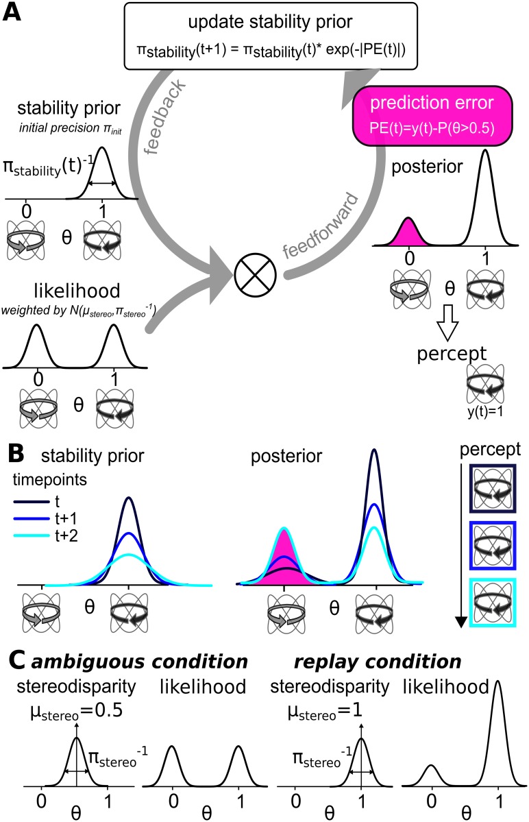
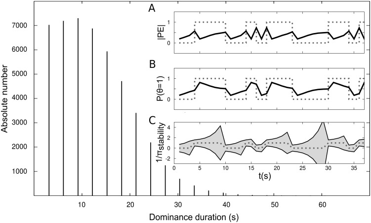
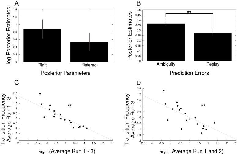
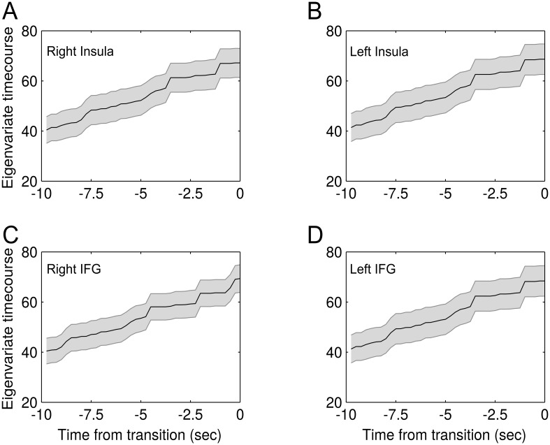
In bistable vision, subjective perception wavers between two interpretations of a constant ambiguous stimulus. This dissociation between conscious perception and sensory stimulation has motivated various empirical studies on the neural correlates of bistable perception, but the neurocomputational mechanism behind endogenous perceptual transitions has remained elusive. Here, we recurred to a generic Bayesian framework of predictive coding and devised a model that casts endogenous perceptual transitions as a consequence of prediction errors emerging from residual evidence for the suppressed percept. Data simulations revealed close similarities between the model's predictions and key temporal characteristics of perceptual bistability, indicating that the model was able to reproduce bistable perception. Fitting the predictive coding model to behavioural data from an fMRI-experiment on bistable perception, we found a correlation across participants between the model parameter encoding perceptual stabilization and the behaviourally measured frequency of perceptual transitions, corroborating that the model successfully accounted for participants' perception. Formal model comparison with established models of bistable perception based on mutual inhibition and adaptation, noise or a combination of adaptation and noise was used for the validation of the predictive coding model against the established models. Most importantly, model-based analyses of the fMRI data revealed that prediction error time-courses derived from the predictive coding model correlated with neural signal time-courses in bilateral inferior frontal gyri and anterior insulae. Voxel-wise model selection indicated a superiority of the predictive coding model over conventional analysis approaches in explaining neural activity in these frontal areas, suggesting that frontal cortex encodes prediction errors that mediate endogenous perceptual transitions in bistable perception. Taken together, our current work provides a theoretical framework that allows for the analysis of behavioural and neural data using a predictive coding perspective on bistable perception. In this, our approach posits a crucial role of prediction error signalling for the resolution of perceptual ambiguities.
Overview
The claims and statistics of this paper haven’t been checked yet.
Free: it reads the open-access text and checks the first 5 claims that cite a source we can check. Create a free account to check every claim.
Integrity signals
Registry
Cites
Statistics
Figures

Verification
Claims the paper makes
The claims and statistics of this paper haven’t been checked yet.
Free: it reads the open-access text and checks the first 5 claims that cite a source we can check. Create a free account to check every claim.
Claims other papers make about this one
Each is checked against this paper’s own text: does it say what the citing paper says it does?
The cited source says what the claim attributes to it.
In the citing paper
“The explanatory power of this framework, exemplified in simulations of PP that readily account for phenomena ranging from V1 neuron response properties 207 to bistable perception 29 to perceptual illusions, 30 , 31 has led some to argue that everything the brain does can ultimately be explained in terms of prediction error minimization.”
From Evaluating the neurophysiological evidence for predictive processing as a model of perception (2020) · cites this paper as [29]
Self-check
Percentages, sums and reported differences re-computed from the paper’s own numbers.
The self-check needs the paper’s full text.
Citations
Cites
Brainard, D. H. (1997) · Spatial Vision · doi:10.1163/156856897x00357 · Cited by 19,702
The free-energy principle: a unified brain theory?
Friston, K. (2010) · Nature Reviews Neuroscience · doi:10.1038/nrn2787 · Cited by 8,120
Whatever next? Predictive brains, situated agents, and the future of cognitive science
Clark, A. (2013) · Behavioral and Brain Sciences · doi:10.1017/s0140525x12000477 · Cited by 5,924
Rao, R. P. N., & Ballard, D. H. (1999) · Nature Neuroscience · doi:10.1038/4580 · Cited by 5,483
A theory of cortical responses.
Friston, K. (2005) · Philosophical Transactions of the Royal Society B: Biological Sciences · doi:10.1098/rstb.2005.1622 · Cited by 4,578
A new SPM toolbox for combining probabilistic cytoarchitectonic maps and functional imaging data
Eickhoff, S. B., Stephan, K. E., Mohlberg, H., Grefkes, C., Fink, G. R., Amunts, K., & Zilles, K. (2005) · NeuroImage · doi:10.1016/j.neuroimage.2004.12.034 · Cited by 4,033
The Bayesian brain: The role of uncertainty in neural coding and computation
Knill, D. C., & Pouget, A. (2004) · Trends in Neurosciences · doi:10.1016/j.tins.2004.10.007 · Cited by 2,588
Hierarchical Bayesian inference in the visual cortex
Lee, T. S., & Mumford, D. (2003) · Journal of the Optical Society of America A · doi:10.1364/josaa.20.001434 · Cited by 1,473
Bayesian model selection for group studies
Stephan, K. E., Penny, W. D., Daunizeau, J., Moran, R. J., & Friston, K. J. (2009) · NeuroImage · doi:10.1016/j.neuroimage.2009.03.025 · Cited by 1,423
Multistable phenomena: changing views in perception
Leopold, D. A., & Logothetis, N. K. (1999) · Trends in Cognitive Sciences · doi:10.1016/s1364-6613(99)01332-7 · Cited by 962
Serial dependence in visual perception
Fischer, J., & Whitney, D. (2014) · Nature Neuroscience · doi:10.1038/nn.3689 · Cited by 806
Neural Correlates of Perceptual Rivalry in the Human Brain
Lumer, E. D., Friston, K. J., & Rees, G. (1998) · Science · doi:10.1126/science.280.5371.1930 · Cited by 745
Neural bases of binocular rivalry
Tong, F., Meng, M., & Blake, R. (2006) · Trends in Cognitive Sciences · doi:10.1016/j.tics.2006.09.003 · Cited by 691
Friston, K. J., & Stephan, K. E. (2007) · Synthese · doi:10.1007/s11229-007-9237-y · Cited by 673
What is rivalling during binocular rivalry?
Logothetis, N. K., Leopold, D. A., & Sheinberg, D. L. (1996) · Nature · doi:10.1038/380621a0 · Cited by 560
Predictive coding explains binocular rivalry: an epistemological review
Hohwy, J., Roepstorff, A., & Friston, K. (2008) · Cognition · doi:10.1016/j.cognition.2008.05.010 · Cited by 546
Model‐Based fMRI and Its Application to Reward Learning and Decision Making
O'DOHERTY, J. P., HAMPTON, A., & KIM, H. (2007) · Annals of the New York Academy of Sciences · doi:10.1196/annals.1390.022 · Cited by 508
Uncertainty in perception and the Hierarchical Gaussian Filter
Mathys, C. D., Lomakina, E. I., Daunizeau, J., Iglesias, S., Brodersen, K. H., Friston, K. J., & Stephan, K. E. (2014) · Frontiers in Human Neuroscience · doi:10.3389/fnhum.2014.00825 · Cited by 465
Binocular rivalry: frontal activity relates to introspection and action but not to perception
Frässle, S., Sommer, J., Jansen, A., Naber, M., & Einhäuser, W. (2014) · The Journal of Neuroscience · doi:10.1523/jneurosci.4403-13.2014 · Cited by 409
The neural bases of multistable perception
Sterzer, P., Kleinschmidt, A., & Rees, G. (2009) · Trends in Cognitive Sciences · doi:10.1016/j.tics.2009.04.006 · Cited by 399
Self-citationAttention and conscious perception in the hypothesis testing brain
Hohwy, J. (2012) · Frontiers in Psychology · doi:10.3389/fpsyg.2012.00096 · Cited by 396
Noise-Induced Alternations in an Attractor Network Model of Perceptual Bistability
Moreno-Bote, R., Rinzel, J., & Rubin, N. (2007) · Journal of Neurophysiology · doi:10.1152/jn.00116.2007 · Cited by 378
An Astable Multivibrator Model of Binocular Rivalry
Lehky, S. R. (1988) · Perception · doi:10.1068/p170215 · Cited by 260
The time course of binocular rivalry reveals a fundamental role of noise
Brascamp, J. W., van Ee, R., Noest, A. J., Jacobs, R. H. A. H., & van den Berg, A. V. (2006) · Journal of Vision · doi:10.1167/6.11.8 · Cited by 232
The Role of Frontal and Parietal Brain Areas in Bistable Perception
Knapen, T., Brascamp, J., Pearson, J., van Ee, R., & Blake, R. (2011) · Journal of Neuroscience · doi:10.1523/jneurosci.1727-11.2011 · Cited by 210
Sensory memory for ambiguous vision
Pearson, J., & Brascamp, J. (2008) · Trends in Cognitive Sciences · doi:10.1016/j.tics.2008.05.006 · Cited by 198
Serial Dependence in Perceptual Decisions Is Reflected in Activity Patterns in Primary Visual Cortex
St. John-Saaltink, E., Kok, P., Lau, H. C., & de Lange, F. P. (2016) · The Journal of Neuroscience · doi:10.1523/jneurosci.4390-15.2016 · Cited by 191
A neural basis for inference in perceptual ambiguity
Sterzer, P., & Kleinschmidt, A. (2007) · Proceedings of the National Academy of Sciences · doi:10.1073/pnas.0609006104 · Cited by 186
Self-citationMinimal physiological conditions for binocular rivalry and rivalry memory
Wilson, H. R. (2007) · Vision Research · doi:10.1016/j.visres.2007.07.007 · Cited by 173
NOTE ON THE DISTRIBUTION OF DOMINANCE TIMES IN BINOCULAR RIVALRY
LEVELT, W. J. M. (1967) · British Journal of Psychology · doi:10.1111/j.2044-8295.1967.tb01068.x · Cited by 170
Negligible fronto-parietal BOLD activity accompanying unreportable switches in bistable perception
Brascamp, J., Blake, R., & Knapen, T. (2015) · Nature Neuroscience · doi:10.1038/nn.4130 · Cited by 159
Structural and functional fractionation of right superior parietal cortex in bistable perception
Kanai, R., Carmel, D., Bahrami, B., & Rees, G. (2011) · Current Biology · doi:10.1016/j.cub.2010.12.009 · Cited by 126
Perceptual multistability predicted by search model for bayesian decisions.
Sundareswara, R., & Schrater, P. R. (2008) · Journal of Vision · doi:10.1167/8.5.12 · Cited by 112
Klink, P. C., van Ee, R., Nijs, M. M., Brouwer, G. J., Noest, A. J., & Wezel, R. J. A. V. (2008) · Journal of Vision · doi:10.1167/8.5.16 · Cited by 102
Frontoparietal Cortex Mediates Perceptual Transitions in Bistable Perception
Weilnhammer, V. A., Ludwig, K., Hesselmann, G., & Sterzer, P. (2013) · The Journal of Neuroscience · doi:10.1523/jneurosci.1418-13.2013 · Cited by 80
Self-citationBayesian model selection maps for group studies
Rosa, M. J., Bestmann, S., Harrison, L., & Penny, W. (2010) · NeuroImage · doi:10.1016/j.neuroimage.2009.08.051 · Cited by 74
Brain activity dynamics in human parietal regions during spontaneous switches in bistable perception
Megumi, F., Bahrami, B., Kanai, R., & Rees, G. E. (2014) · NeuroImage · doi:10.1016/j.neuroimage.2014.12.018 · Cited by 63
A very inexpensive MRI-compatible method for dichoptic visual stimulation
Schurger, A. (2008) · Journal of Neuroscience Methods · doi:10.1016/j.jneumeth.2008.09.028 · Cited by 56
Believable change: Bistable reversals are governed by physical plausibility
Pastukhov, A., Vonau, V., & Braun, J. (2012) · Journal of Vision · doi:10.1167/12.1.17 · Cited by 41
Revisiting the Lissajous figure as a tool to study bistable perception
Weilnhammer, V. A., Ludwig, K., Sterzer, P., & Hesselmann, G. (2014) · Vision Research · doi:10.1016/j.visres.2014.03.013 · Cited by 15
Self-citationPanagiotaropoulos, T. I., Kapoor, V., Logothetis, N. K., & Deco, G. (2013) · PLoS ONE · doi:10.1371/journal.pone.0053833 · Cited by 14
Perceptual Stability of the Lissajous Figure Is Modulated by the Speed of Illusory Rotation
Weilnhammer, V. A., Sterzer, P., & Hesselmann, G. (2016) · PLoS ONE · doi:10.1371/journal.pone.0160772 · Cited by 8
Self-citation
Cited by
Evaluating the neurophysiological evidence for predictive processing as a model of perception
Walsh, K. S., McGovern, D. P., Clark, A., & O'Connell, R. G. (2020) · Annals of the New York Academy of Sciences · doi:10.1111/nyas.14321 · Cited by 333
New directions in predictive processing
Hohwy, J. (2020) · Mind & Language · doi:10.1111/mila.12281 · Cited by 247
“That optimism now seems somewhat vindicated in light of recent empirical evidence and computational models (Weilnhammer et al., 2017, Parr et al., 2019).”
BackgroundPredictive processing as a systematic basis for identifying the neural correlates of consciousness
Hohwy, J., & Seth, A. (2020) · Philosophy and the Mind Sciences · doi:10.33735/phimisci.2020.ii.64 · Cited by 170
Multistable Perception and the Role of the Frontoparietal Cortex in Perceptual Inference
Brascamp, J., Sterzer, P., Blake, R., & Knapen, T. (2018) · Annual Review of Psychology · doi:10.1146/annurev-psych-010417-085944 · Cited by 164
Self-citationIllusory Motion Reproduced by Deep Neural Networks Trained for Prediction
Watanabe, E., Kitaoka, A., Sakamoto, K., Yasugi, M., & Tanaka, K. (2018) · Frontiers in Psychology · doi:10.3389/fpsyg.2018.00345 · Cited by 101
“…to generate illusions (Notredame et al., 2014; Nour and Nour, 2015; Raman and Sarkar, 2016; Shipp, 2016) and was used as an explanation for certain motion illusions (Watanabe et al., 2010), of bi-stable perception (Weilnhammer et al., 2017) and of an apparent motion illusion (Edwards et al., 2017).”
BackgroundMethod
Metadata
- Authors
- Weilnhammer, V., Stuke, H., Hesselmann, G., Sterzer, P., & Schmack, K.
- Affiliations
- Charité – Universitätsmedizin Berlin (DE)
- Humboldt-Universität zu Berlin (DE)
- Corresponding author
- Weilnhammer, Veith
- Venue
- PLOS Computational Biology
- Publisher
- Public Library of Science (PLoS)
- Published
- 2017-05-15
- Volume
- 13
- Issue
- 5
- Pages
- e1005536
- ISSN
- 1553-734X (ISSN-L)
- 1553-7358
- PMC
- PMC5448813
- OpenAlex
- W2615931912
- Cited by
- 120
- References
- 43
- Citations by year
- 2026: 12 · 2025: 13 · 2024: 12 · 2023: 12 · 2022: 12 · 2021: 15 · 2020: 24 · 2019: 5 · 2018: 10 · 2017: 5
- FWCI
- 6.91
- Type
- journal article
- Language
- en
- Update notices
- new_version (2017-05-30)
- Open access
- gold
- doi.org
- Licence
- Locations
- PLoS Computational Biology (publishedVersion, cc-by)
- Europe PMC (PubMed Central) (publishedVersion, cc-by)
- PubMed Central (publishedVersion, cc-by)
- PubMed (publishedVersion)
- RePEc: Research Papers in Economics (submittedVersion)
- DOAJ (DOAJ: Directory of Open Access Journals) (submittedVersion, cc-by-sa)
- Figshare (submittedVersion, cc-by)
- Refubium (Universitätsbibliothek der Freien Universität Berlin) (submittedVersion, cc-by)
- Universitätsbibliothek der FU Berlin Hochschulschriftenstelle u. Dokumentenserver (cc-by)
- Funders
- e:Med research and funding concept (01ZX1404A)
- German Research Foundation (HE 6244/1-2, STE 1430/7-1)
- Charité Clinical Scientist Program
- Charité Junior Clinical Scientist Program
- Topics
- Life Sciences › Neuroscience › Cognitive Neuroscience › Visual perception and processing mechanisms
- Life Sciences › Neuroscience › Cognitive Neuroscience › Embodied and Extended Cognition
- Social Sciences › Arts and Humanities › Philosophy › Philosophy and Theoretical Science
- Keywords
- bistable perception, predictive coding, prediction error, perceptual transitions, perceptual stabilization, Bayesian model, inferior frontal gyrus, anterior insula, model-based fMRI, model comparison, reciprocal inhibition, adaptation, noise
- MeSH terms
- Adult, Bayes Theorem, Computer Simulation, Female, Frontal Lobe, Humans, Magnetic Resonance Imaging, Male, Models, Neurological, Task Performance and Analysis, Visual Perception, Computational Biology, Young Adult
About these checks
Registry, retraction, Cites and statistics results are computed, not judged, with one exception: a printed reference that no index lists is read once by a model before it counts as a citation error. Claims are extracted by a model and kept only when their quote appears verbatim in the text; each cited source is then checked, with a model’s help, for whether it says what the claim relies on. Those verdicts can be wrong — read the claim’s quote and the cited source before relying on one.
Statistics and arithmetic are recomputed, not judged.
Confidence bands are shown only for fields calibrated on our annotated test set. None is calibrated yet, so no band is shown.
What counts as a claim ›How we measure confidence ›How we check this ›
Are you an author, or do you see a problem with this page? Request a review
Data sources
Bibliographic data: Semantic Scholar, OpenAlex, Crossref.
Contains information from the Semantic Scholar Academic Graph Datasets, made available under the ODC Attribution License (ODC-BY 1.0).
Semantic Scholar’s data is described in: Kinney, R., et al. (2023). The Semantic Scholar Open Data Platform. arXiv:2301.10140.
