

The DOI matches its Crossref record; 116 of the 120 references it cites were found in a registry or an index.
RosettaAntibodyDesign (RAbD): A general framework for computational antibody design
Open accessPublished version of a preprint
Abstract
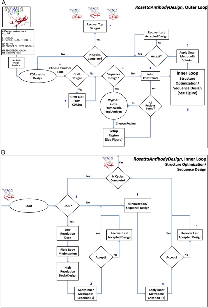
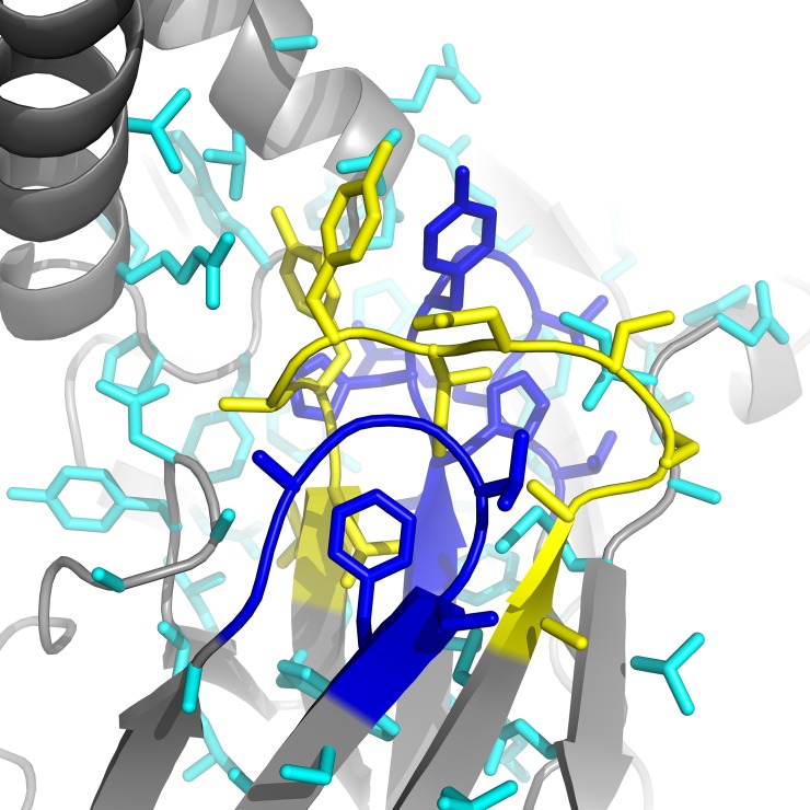
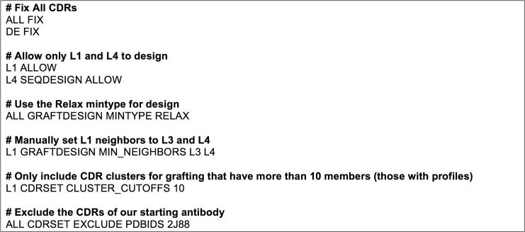
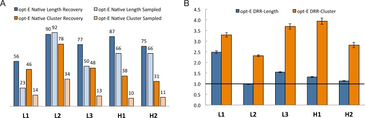
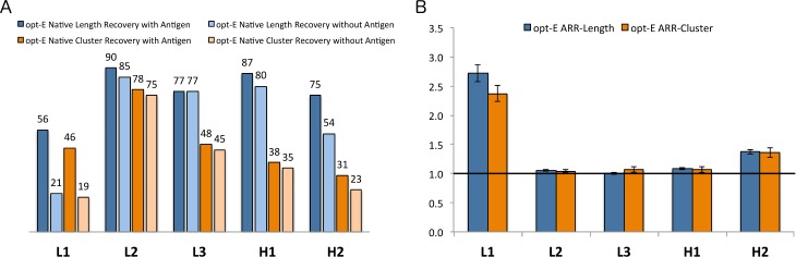
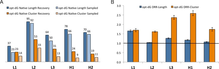
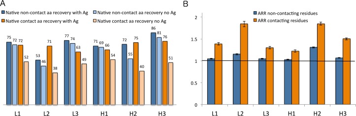
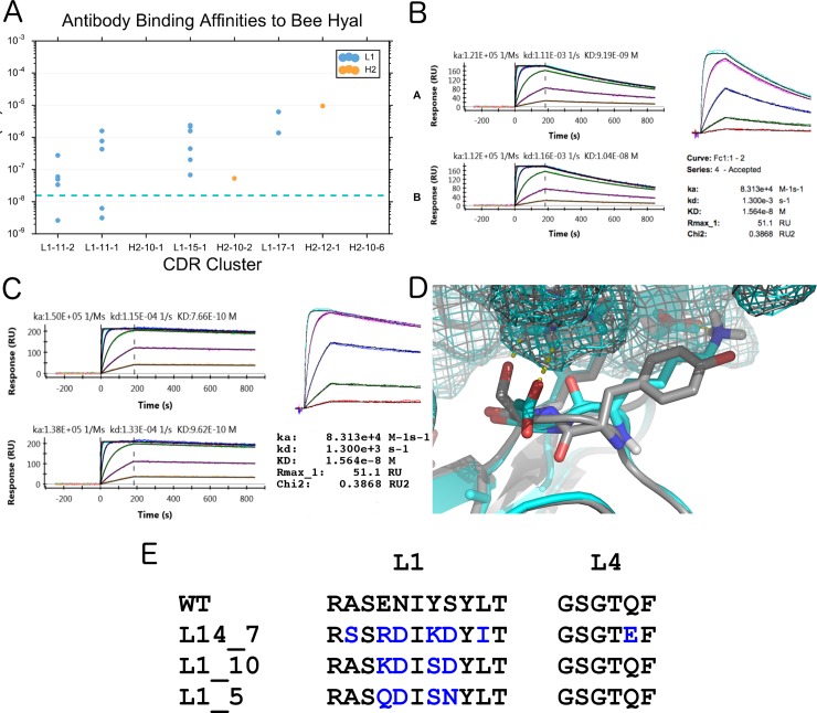
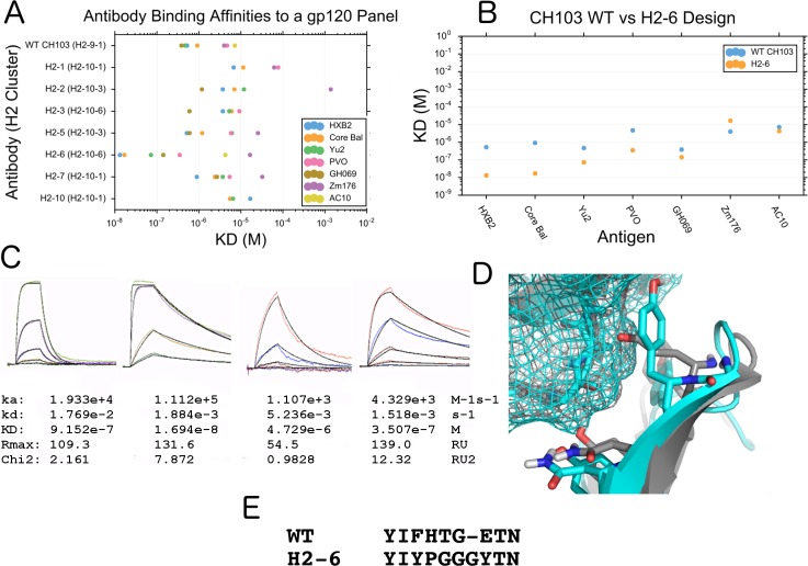
A structural-bioinformatics-based computational methodology and framework have been developed for the design of antibodies to targets of interest. RosettaAntibodyDesign (RAbD) samples the diverse sequence, structure, and binding space of an antibody to an antigen in highly customizable protocols for the design of antibodies in a broad range of applications. The program samples antibody sequences and structures by grafting structures from a widely accepted set of the canonical clusters of CDRs (North et al., J. Mol. Biol., 406:228-256, 2011). It then performs sequence design according to amino acid sequence profiles of each cluster, and samples CDR backbones using a flexible-backbone design protocol incorporating cluster-based CDR constraints. Starting from an existing experimental or computationally modeled antigen-antibody structure, RAbD can be used to redesign a single CDR or multiple CDRs with loops of different length, conformation, and sequence. We rigorously benchmarked RAbD on a set of 60 diverse antibody-antigen complexes, using two design strategies-optimizing total Rosetta energy and optimizing interface energy alone. We utilized two novel metrics for measuring success in computational protein design. The design risk ratio (DRR) is equal to the frequency of recovery of native CDR lengths and clusters divided by the frequency of sampling of those features during the Monte Carlo design procedure. Ratios greater than 1.0 indicate that the design process is picking out the native more frequently than expected from their sampled rate. We achieved DRRs for the non-H3 CDRs of between 2.4 and 4.0. The antigen risk ratio (ARR) is the ratio of frequencies of the native amino acid types, CDR lengths, and clusters in the output decoys for simulations performed in the presence and absence of the antigen. For CDRs, we achieved cluster ARRs as high as 2.5 for L1 and 1.5 for H2. For sequence design simulations without CDR grafting, the overall recovery for the native amino acid types for residues that contact the antigen in the native structures was 72% in simulations performed in the presence of the antigen and 48% in simulations performed without the antigen, for an ARR of 1.5. For the non-contacting residues, the ARR was 1.08. This shows that the sequence profiles are able to maintain the amino acid types of these conserved, buried sites, while recovery of the exposed, contacting residues requires the presence of the antigen-antibody interface. We tested RAbD experimentally on both a lambda and kappa antibody-antigen complex, successfully improving their affinities 10 to 50 fold by replacing individual CDRs of the native antibody with new CDR lengths and clusters.
Overview
The claims and statistics of this paper haven’t been checked yet.
Run the check — free, no account needed. It reads the open-access text and checks the sources it cites.
Integrity signals
Registry
Cites
Statistics
Figures
Verification
Claims the paper makes
The claims and statistics of this paper haven’t been checked yet.
Run the check — free, no account needed. It reads the open-access text and checks the sources it cites.
Claims other papers make about this one
Each is checked against this paper’s own text: does it say what the citing paper says it does?
In the citing paper
“RosettaAntibodyDesign (RAbD) [89] relies on two algorithmic loops referred to the outer and inner loops of design.”
From Computational and artificial intelligence-based methods for antibody development (2023) · cites this paper as [89]
Self-check
Percentages, sums and reported differences re-computed from the paper’s own numbers.
The self-check needs the paper’s full text.
Citations
Cites
Gentleman R: R: A language for data analysis and graphics
Ihaka, R., & Gentleman, R. (1996) · Journal of Computational and Graphical Statistics · doi:10.1080/10618600.1996.10474713 · Cited by 11,747
Amino acid substitution matrices from protein blocks.
Henikoff, S., & Henikoff, J. G. (1992) · Proceedings of the National Academy of Sciences · doi:10.1073/pnas.89.22.10915 · Cited by 6,218
R: A Language for Data Analysis and Graphics
Ihaka, R., & Gentleman, R. C. (1996) · Journal of Computational and Graphical Statistics · doi:10.2307/1390807 · Cited by 4,245
Smith, G. P. (1985) · Science · doi:10.1126/science.4001944 · Cited by 4,143
Phage antibodies: filamentous phage displaying antibody variable domains
McCafferty, J., Griffiths, A. D., Winter, G. P., & Chiswell, D. J. (1990) · Nature · doi:10.1038/348552a0 · Cited by 2,427
Engineered antibody fragments and the rise of single domains
Holliger, P., & Hudson, P. J. (2005) · Nature Biotechnology · doi:10.1038/nbt1142 · Cited by 1,928
Design of a Novel Globular Protein Fold with Atomic-Level Accuracy
Kuhlman, B. A., Dantas, G. A., Ireton, G. C., Varani, G., Stoddard, B. L., & Baker, D. A. (2003) · Science · doi:10.1126/science.1089427 · Cited by 1,666
Making antibodies by phage display technology
Winter, G., Griffiths, A. D., Hawkins, R. E., & Hoogenboom, H. R. (1994) · Annual Review of Immunology · doi:10.1146/annurev.iy.12.040194.002245 · Cited by 1,573
The Rosetta All-Atom Energy Function for Macromolecular Modeling and Design
Alford, R. F., Leaver-Fay, A., Jeliazkov, J. R., O’Meara, M. J., DiMaio, F. P., Park, H., Shapovalov, M. V., Renfrew, P. D., Mulligan, V. K., Kappel, K., et al. (2017) · Journal of Chemical Theory and Computation · doi:10.1021/acs.jctc.7b00125 · Cited by 1,532
Self-citationCanonical structures for the hypervariable regions of immunoglobulins
Chothia, C., & Lesk, A. M. (1987) · Journal of Molecular Biology · doi:10.1016/0022-2836(87)90412-8 · Cited by 1,406
Kemp elimination catalysts by computational enzyme design
Röthlisberger, D., Khersonsky, O., Wollacott, A. M., Jiang, L., DeChancie, J., Betker, J. L., Gallaher, J. L., Althoff, E. A., Zanghellini, A., Dym, O., et al. (2008) · Nature · doi:10.1038/nature06879 · Cited by 1,299
Monoclonal antibody therapy of cancer
Adams, G. P., & Weiner, L. M. (2005) · Nature Biotechnology · doi:10.1038/nbt1137 · Cited by 1,272
Shape Complementarity at Protein/Protein Interfaces
Lawrence, M. C., & Colman, P. M. (1993) · Journal of Molecular Biology · doi:10.1006/jmbi.1993.1648 · Cited by 1,224
Making antibody fragments using phage display libraries
Clackson, T., Hoogenboom, H. R., Griffiths, A. D., & Winter, G. P. (1991) · Nature · doi:10.1038/352624a0 · Cited by 1,211
Shape complementarity at protein–protein interfaces
Norel, R., Lin, S. L., Wolfson, H. J., & Nussinov, R. (1994) · Biopolymers · doi:10.1002/bip.360340711 · Cited by 1,208
De Novo Computational Design of Retro-Aldol Enzymes
Jiang, L., Althoff, E. A., Clemente, F. R., Doyle, L., Röthlisberger, D., Zanghellini, A., Gallaher, J. L., Betker, J. L., Tanaka, F., Barbas, C. F., et al. (2008) · Science · doi:10.1126/science.1152692 · Cited by 1,174
Gray, J. J., Moughon, S. E., Wang, C., Schueler‐Furman, O., Kuhlman, B. A., Rohl, C. A., & Baker, D. A. (2003) · Journal of Molecular Biology · doi:10.1016/s0022-2836(03)00670-3 · Cited by 1,130
Arming antibodies: prospects and challenges for immunoconjugates
Wu, A. M., & Senter, P. D. (2005) · Nature Biotechnology · doi:10.1038/nbt1141 · Cited by 1,053
Shapovalov, M. V., & Dunbrack, R. L. (2011) · Structure · doi:10.1016/j.str.2011.03.019 · Cited by 1,000
Self-citationMacromolecular Modeling with Rosetta
Das, R., & Baker, D. A. (2008) · Annual Review of Biochemistry · doi:10.1146/annurev.biochem.77.062906.171838 · Cited by 995
Davies, H. T. O., Crombie, I. K., & Tavakoli, M. (1998) · BMJ · doi:10.1136/bmj.316.7136.989 · Cited by 991
Co-evolution of a broadly neutralizing HIV-1 antibody and founder virus
Liao, H., Lynch, R. M., Zhou, T., Gao, F., Alam, S. M., Boyd, S. D., Fire, A. Z., Roskin, K. M., Schramm, C. A., Zhang, Z., et al. (2013) · Nature · doi:10.1038/nature12053 · Cited by 986
Human cancer immunotherapy with antibodies to the PD-1 and PD-L1 pathway
Ohaegbulam, K. C., Assal, A., Lázár‐Molnár, E., Yao, Y., & Zang, X. (2014) · Trends in Molecular Medicine · doi:10.1016/j.molmed.2014.10.009 · Cited by 861
Bayesian statistical analysis of protein side‐chain rotamer preferences
Dunbrack, R. L., & Cohen, F. E. (1997) · Protein Science · doi:10.1002/pro.5560060807 · Cited by 776
Self-citationPyRosetta: a script-based interface for implementing molecular modeling algorithms using Rosetta
Chaudhury, S., Lyskov, S., & Gray, J. J. (2010) · Bioinform. · doi:10.1093/bioinformatics/btq007 · Cited by 772
The biotin-(strept)avidin system: principles and applications in biotechnology
Diamandis, E. P., & Christopoulos, T. K. (1991) · Clinical Chemistry · doi:10.1093/clinchem/37.5.625 · Cited by 748
Antibody Multispecificity Mediated by Conformational Diversity
James, L. C., Roversi, P., & Tawfik, D. S. (2003) · Science · doi:10.1126/science.1079731 · Cited by 719
Standard conformations for the canonical structures of immunoglobulins 1 1Edited by I. A. Wilson
Al‐Lazikani, B., Lesk, A. M., & Chothia, C. (1997) · Journal of Molecular Biology · doi:10.1006/jmbi.1997.1354 · Cited by 707
RosettaScripts: A Scripting Language Interface to the Rosetta Macromolecular Modeling Suite
Fleishman, S. J., Leaver‐Fay, A., Corn, J. E., Strauch, E., Khare, S. D., Koga, N., Ashworth, J. R., Murphy, P. M., Richter, F. M., Lemmon, G., et al. (2011) · PLoS ONE · doi:10.1371/journal.pone.0020161 · Cited by 659
Adams, G. P., Schier, R., McCall, A. M., Simmons, H. H., Horak, E. M., Alpaugh, R. K., Marks, J. D., & Weiner, L. M. (2001) · PubMed · Cited by 623
Design of therapeutic proteins with enhanced stability
Chennamsetty, N., Voynov, V., Kayser, V., Helk, B., & Trout, B. L. (2009) · Proceedings of the National Academy of Sciences · doi:10.1073/pnas.0904191106 · Cited by 605
Computational Design of Proteins Targeting the Conserved Stem Region of Influenza Hemagglutinin
Fleishman, S. J., Whitehead, T. A., Ekiert, D. C., Dreyfus, C., Corn, J. E., Strauch, E.-M., Wilson, I. A., & Baker, D. (2011) · Science · doi:10.1126/science.1202617 · Cited by 585
Cyclic coordinate descent: A robotics algorithm for protein loop closure
Canutescu, A. A., & Dunbrack, R. L. (2003) · Protein Science · doi:10.1110/ps.0242703 · Cited by 527
Self-citationSelection of phage antibodies by binding affinity
Hawkins, R. E., Russell, S. J., & Winter, G. P. (1992) · Journal of Molecular Biology · doi:10.1016/0022-2836(92)90639-2 · Cited by 526
IMGT®, the international ImMunoGeneTics information system®
Lefranc, M., Giudicelli, V., Ginestoux, C., Jabado-Michaloud, J., Folch, G., Bellahcene, F., Wu, Y., Gemrot, E., Brochet, X., Lane, J., et al. (2004) · Nucleic Acids Res. · doi:10.1093/nar/gkn838 · Cited by 521
Broadly Neutralizing Antiviral Antibodies
Corti, D., & Lanzavecchia, A. (2013) · Annual Review of Immunology · doi:10.1146/annurev-immunol-032712-095916 · Cited by 469
Sub-angstrom accuracy in protein loop reconstruction by robotics-inspired conformational sampling
Mandell, D. J., Coutsias, E. A., & Kortemme, T. (2009) · Nature Methods · doi:10.1038/nmeth0809-551 · Cited by 458
Protein–Protein Docking with Backbone Flexibility
Wang, C., Bradley, P. H., & Baker, D. A. (2007) · Journal of Molecular Biology · doi:10.1016/j.jmb.2007.07.050 · Cited by 420
Alternate States of Proteins Revealed by Detailed Energy Landscape Mapping
Tyka, M. D., Keedy, D. A., André, I., DiMaio, F., Song, Y., Richardson, D. C., Richardson, J. S., & Baker, D. A. (2010) · Journal of Molecular Biology · doi:10.1016/j.jmb.2010.11.008 · Cited by 410
Relaxation of backbone bond geometry improves protein energy landscape modeling
Conway, P., Tyka, M. D., DiMaio, F., Konerding, D. E., & Baker, D. A. (2013) · Protein Science · doi:10.1002/pro.2389 · Cited by 408
A new clustering of antibody CDR loop conformations
North, B., Lehmann, A., & Dunbrack, R. L. (2011) · Journal of Molecular Biology · doi:10.1016/j.jmb.2010.10.030 · Cited by 380
Self-citationYang, L. P. H., Mao, H. Z., Wang, Y. A., Cao, Z., Peng, X., Wang, X., Duan, H., Ni, C., Yuan, Q., Adams, G. P., et al. (2008) · Small · doi:10.1002/smll.200800714 · Cited by 360
De Novo Enzyme Design Using Rosetta3
Richter, F. M., Leaver‐Fay, A., Khare, S. D., Bjelic, S., & Baker, D. A. (2011) · PLoS ONE · doi:10.1371/journal.pone.0019230 · Cited by 359
Computational design of antibody-affinity improvement beyond in vivo maturation
Lippow, S. M., Wittrup, K. D., & Tidor, B. (2007) · Nature Biotechnology · doi:10.1038/nbt1336 · Cited by 342
Morea, V., Tramontano, A. L., Rustici, M., Chothia, C., & Lesk, A. M. (1998) · Journal of Molecular Biology · doi:10.1006/jmbi.1997.1442 · Cited by 327
Smith, C. A., & Kortemme, T. (2008) · Journal of Molecular Biology · doi:10.1016/j.jmb.2008.05.023 · Cited by 314
The Role of Balanced Training and Testing Data Sets for Binary Classifiers in Bioinformatics
Wei, Q., & Dunbrack, R. L. (2013) · PLoS ONE · doi:10.1371/journal.pone.0067863 · Cited by 298
Self-citationA Pareto-Optimal Refinement Method for Protein Design Scaffolds
Nivón, L. G., Moretti, R., & Baker, D. A. (2013) · PLoS ONE · doi:10.1371/journal.pone.0059004 · Cited by 295
IMGT, the International ImMunoGeneTics Information SystemPreprint
Lefranc, M. (2011) · Cold Spring Harbor Protocols · doi:10.1101/pdb.top115 · Cited by 289
Tiller, K. E., & Tessier, P. M. (2015) · Annual Review of Biomedical Engineering · doi:10.1146/annurev-bioeng-071114-040733 · Cited by 270
Modeling and docking of antibody structures with Rosetta
Weitzner, B. D., Jeliazkov, J. R., Lyskov, S., Marze, N. A., Kuroda, D., Frick, R., Adolf‐Bryfogle, J., Biswas, N., Dunbrack, R. L., & Gray, J. J. (2017) · Nature Protocols · doi:10.1038/nprot.2016.180 · Cited by 266
Self-citationThe Backrub Motion: How Protein Backbone Shrugs When a Sidechain Dances
Davis, I., Arendall, W. B., Richardson, D. C., & Richardson, J. S. (2006) · Structure · doi:10.1016/j.str.2005.10.007 · Cited by 264
Honegger, A., & Plückthun, A. (2001) · Journal of Molecular Biology · doi:10.1006/jmbi.2001.4662 · Cited by 249
Martin, A. C. R., & Thornton, J. M. (1996) · Journal of Molecular Biology · doi:10.1006/jmbi.1996.0617 · Cited by 246
Stranges, P. B., & Kuhlman, B. A. (2012) · Protein Science · doi:10.1002/pro.2187 · Cited by 233
Deeks, J. J., Bracken, M. B., Sinclair, J. C., Davies, H. T. O., Tavakoli, M., & Crombie, I. K. (1998) · BMJ · doi:10.1136/bmj.317.7166.1155a · Cited by 225
Computer-aided antibody design
Kuroda, D., Shirai, H., Jacobson, M. P., & Nakamura, H. (2012) · Protein Engineering Design and Selection · doi:10.1093/protein/gzs024 · Cited by 225
Natural and designer binding sites made by phage display technology
Hoogenboom, H. R., & Chames, P. (2000) · Immunology Today · doi:10.1016/s0167-5699(00)01667-4 · Cited by 216
Designing and optimizing library selection strategies for generating high-affinity antibodies
Hoogenboom, H. R. (1997) · Trends in biotechnology · doi:10.1016/s0167-7799(97)84205-9 · Cited by 215
Rational design and engineering of therapeutic proteins
Marshall, S. A., Lazar, G. A., Chirino, A. J., & Desjarlais, J. R. (2003) · Drug Discovery Today · doi:10.1016/s1359-6446(03)02610-2 · Cited by 209
Progress in phage display: evolution of the technique and its applications
Bratkovič, T. (2009) · Cellular and Molecular Life Sciences · doi:10.1007/s00018-009-0192-2 · Cited by 208
Antibody affinity maturation using bacterial surface display
Daugherty, P. S., Chen, G., Olsen, M. J., Iverson, B. L., & Georgiou, G. (1998) · Protein Engineering Design and Selection · doi:10.1093/protein/11.9.825 · Cited by 197
Scientific Benchmarks for Guiding Macromolecular Energy Function Improvement
Leaver‐Fay, A., O’Meara, M. J., Tyka, M., Jacak, R., Song, Y., Kellogg, E. H., Thompson, J., Davis, I., Pache, R. A., Lyskov, S., et al. (2013) · Methods in enzymology on CD-ROM/Methods in enzymology · doi:10.1016/b978-0-12-394292-0.00006-0 · Cited by 193
Clark, L. A., Boriack‐Sjodin, P. A., Eldredge, J. K., Fitch, C., Friedman, B., Hanf, K. J. M., Jarpe, M. B., Liparoto, S. F., Li, Y., Lugovskoy, A. A., et al. (2006) · Protein Science · doi:10.1110/ps.052030506 · Cited by 173
Ponsel, D., Neugebauer, J. K., Ladetzki-Baehs, K., & Tissot, K. (2011) · Molecules · doi:10.3390/molecules16053675 · Cited by 164
RosettaAntibody: antibody variable region homology modeling server
Sircar, A., Kim, E. T., & Gray, J. J. (2009) · Nucleic Acids Research · doi:10.1093/nar/gkp387 · Cited by 161
Nayeem, A., Vila, J. A., & Scheraga, H. A. (1991) · Journal of Computational Chemistry · doi:10.1002/jcc.540120509 · Cited by 150
Affinity maturation of antibodies assisted by in silico modeling
Barderas, R., Desmet, J., Timmerman, P., Meloen, R. H., & Casal, J. I. (2008) · Proceedings of the National Academy of Sciences · doi:10.1073/pnas.0801221105 · Cited by 142
Structure-Based Design of Supercharged, Highly Thermoresistant Antibodies
Miklos, A. E., Kluwe, C., Der, B. S., Pai, S., Sircar, A., Hughes, R. A., Berrondo, M., Xu, J., Codrea, V., Buckley, P. E., et al. (2012) · Chemistry & Biology · doi:10.1016/j.chembiol.2012.01.018 · Cited by 142
Design of structurally distinct proteins using strategies inspired by evolution
Jacobs, T. M., Williams, B., Williams, T., Xu, X., Eletsky, A., Federizon, J., Szyperski, T., & Kuhlman, B. A. (2016) · Science · doi:10.1126/science.aad8036 · Cited by 134
Rapid approximation to molecular surface area via the use of Boolean logic and look‐up tables
Grand, S. M. L., & Merz, K. M. (1993) · Journal of Computational Chemistry · doi:10.1002/jcc.540140309 · Cited by 129
Renfrew, P. D., Choi, E. J., Bonneau, R., & Kuhlman, B. A. (2012) · PLoS ONE · doi:10.1371/journal.pone.0032637 · Cited by 128
Computational design of affinity and specificity at protein–protein interfaces
Karanicolas, J., & Kuhlman, B. A. (2009) · Current Opinion in Structural Biology · doi:10.1016/j.sbi.2009.07.005 · Cited by 126
PyIgClassify: a database of antibody CDR structural classifications
Adolf‐Bryfogle, J., Xu, Q., North, B., Lehmann, A., & Dunbrack, R. L. (2014) · Nucleic Acids Research · doi:10.1093/nar/gku1106 · Cited by 120
Self-citationThe Origin of CDR H3 Structural Diversity
Weitzner, B. D., Dunbrack, R. L., & Gray, J. J. (2015) · Structure · doi:10.1016/j.str.2014.11.010 · Cited by 109
Self-citationLapidoth, G. D., Baran, D., Pszolla, G. M., Norn, C., Alon, A., Tyka, M. D., & Fleishman, S. J. (2015) · Proteins Structure Function and Bioinformatics · doi:10.1002/prot.24779 · Cited by 107
Conformation Dependence of Backbone Geometry in Proteins
Berkholz, D. S., Shapovalov, M. V., Dunbrack, R. L., & Karplus, P. A. (2009) · Structure · doi:10.1016/j.str.2009.08.012 · Cited by 107
Self-citationA molecular immunology approach to antibody humanization and functional optimization
Lazar, G. A., Desjarlais, J. R., Jacinto, J. M., Karki, S., & Hammond, P. W. (2006) · Molecular Immunology · doi:10.1016/j.molimm.2006.09.029 · Cited by 107
Der, B. S., Kluwe, C., Miklos, A. E., Jacak, R., Lyskov, S., Gray, J. J., Georgiou, G., Ellington, A. D., & Kuhlman, B. A. (2013) · PLoS ONE · doi:10.1371/journal.pone.0064363 · Cited by 107
Luginbühl, B., Kanyo, Z. F., Jones, R. M., Fletterick, R. J., Prusiner, S. B., Cohen, F. E., Williamson, R. A., Burton, D. R., & Plückthun, A. (2006) · Journal of Molecular Biology · doi:10.1016/j.jmb.2006.07.027 · Cited by 106
Foldit Standalone: a video game-derived protein structure manipulation interface using Rosetta
Kleffner, R., Flatten, J., Leaver‐Fay, A., Baker, D. A., Siegel, J. B., Khatib, F., & Cooper, S. (2017) · Bioinformatics · doi:10.1093/bioinformatics/btx283 · Cited by 106
Human Antibodies from Transgenic Mice
Lönberg, N., & Huszar, D. (1995) · International Reviews of Immunology · doi:10.3109/08830189509061738 · Cited by 104
Transmembrane channel-like (TMC) genes are required for auditory and vestibular mechanosensation
Kawashima, Y., Kurima, K., Pan, B., Griffith, A. J., & Holt, J. R. (2014) · Pflügers Archiv - European Journal of Physiology · doi:10.1007/s00424-014-1582-3 · Cited by 102
Schueler‐Furman, O., Wang, C., & Baker, D. A. (2005) · Proteins Structure Function and Bioinformatics · doi:10.1002/prot.20556 · Cited by 99
The hybridoma revolution: an offshoot of basic research
Milstein, C. (1999) · BioEssays · doi:10.1002/(sici)1521-1878(199911)21:11 · Cited by 97
Pantazes, R. J., & Maranas, C. D. (2010) · Protein Engineering Design and Selection · doi:10.1093/protein/gzq061 · Cited by 97
Weitzner, B. D., Kuroda, D., Marze, N. A., Xu, J., & Gray, J. J. (2014) · Proteins Structure Function and Bioinformatics · doi:10.1002/prot.24534 · Cited by 94
Self-citationHuman Monoclonal Antibodies from Transgenic Mice
Lönberg, N. (2007) · Handbook of experimental pharmacology · doi:10.1007/978-3-540-73259-4_4 · Cited by 90
Prediction of amino acid sequence from structure
Raha, K., Wollacott, A. M., Italia, M. J., & Desjarlais, J. R. (2000) · Protein Science · doi:10.1110/ps.9.6.1106 · Cited by 88
Epidemiology Kept Simple: An Introduction to Traditional and Modern Epidemiology
Gerstman, B. B. (2013) · Cited by 87
Better library design: data‐driven protein engineering
Chaparro‐Riggers, J. F., Polizzi, K. M., & Bommarius, B. (2006) · Biotechnology Journal · doi:10.1002/biot.200600170 · Cited by 87
Padavattan, S., Schirmer, T., Schmidt, M., Akdiş, C. A., Valenta, R., Mittermann, I., Soldatova, L. N., Slater, J. E., Mueller, U. R., & Marković-Housley, Z. (2007) · Journal of Molecular Biology · doi:10.1016/j.jmb.2007.02.036 · Cited by 86
Li, T., Pantazes, R. J., & Maranas, C. D. (2014) · PLoS ONE · doi:10.1371/journal.pone.0105954 · Cited by 79
Computational Design of a PAK1 Binding Protein
Jha, R. K., Leaver‐Fay, A., Yin, S., Wu, Y., Butterfoss, G. L., Szyperski, T., Dokholyan, N. V., & Kuhlman, B. A. (2010) · Journal of Molecular Biology · doi:10.1016/j.jmb.2010.05.006 · Cited by 68
Engineering a protein–protein interface using a computationally designed library
Guntas, G., Purbeck, C., & Kuhlman, B. A. (2010) · Proceedings of the National Academy of Sciences · doi:10.1073/pnas.1006528107 · Cited by 67
SwiftLib: rapid degenerate-codon-library optimization through dynamic programming
Jacobs, T. M., Yumerefendi, H., Kuhlman, B. A., & Leaver‐Fay, A. (2014) · Nucleic Acids Research · doi:10.1093/nar/gku1323 · Cited by 65
Anchored Design of Protein-Protein Interfaces
Lewis, S. M., & Kuhlman, B. A. (2011) · PLoS ONE · doi:10.1371/journal.pone.0020872 · Cited by 64
Hotspot-Centric De Novo Design of Protein Binders
Fleishman, S. J., Corn, J. E., Strauch, E., Whitehead, T. A., Karanicolas, J., & Baker, D. A. (2011) · Journal of Molecular Biology · doi:10.1016/j.jmb.2011.09.001 · Cited by 50
Humanization and molecular modeling of the anti-CD4 monoclonal antibody, OKT4A
Pulito, V. L., Roberts, V., Adair, J. R., Rothermel, A. L., Collins, A., Varga, S. S., Martocello, C., Bodmer, M., Jolliffe, L. K., & Zivin, R. A. (1996) · The Journal of Immunology · doi:10.4049/jimmunol.156.8.2840 · Cited by 48
Computational Design of the Sequence and Structure of a Protein-Binding Peptide
Sammond, D. W., Bosch, D. E., Butterfoss, G. L., Purbeck, C., Machius, M., Siderovski, D. P., & Kuhlman, B. A. (2011) · Journal of the American Chemical Society · doi:10.1021/ja110296z · Cited by 48
Weitzner, B. D., & Gray, J. J. (2016) · The Journal of Immunology · doi:10.4049/jimmunol.1601137 · Cited by 45
Self-citationActivity of 8F4, a T-cell receptor-like anti-PR1/HLA-A2 antibody, against primary human AML in vivo
Сергеева, А., He, H., Ruisaard, K. E., John, L. S. S., Alatrash, G., Clise-Dwyer, K., Li, D., Patenia, R. S., Hong, R., Sukhumalchandra, P., et al. (2016) · Leukemia · doi:10.1038/leu.2016.57 · Cited by 36
Computational de novo design of antibodies binding to a peptide with high affinity
Poosarla, V. G., Li, T., Goh, B. C., Schulten, K. J., Wood, T. K., & Maranas, C. D. (2017) · Biotechnology and Bioengineering · doi:10.1002/bit.26244 · Cited by 36
Lehmann, A., Wixted, J. H. F., Shapovalov, M. V., Röder, H., Dunbrack, R. L., & Robinson, M. K. (2015) · mAbs · doi:10.1080/19420862.2015.1088618 · Cited by 34
Self-citationThe PyRosetta Toolkit: A Graphical User Interface for the Rosetta Software Suite
Adolf‐Bryfogle, J., & Dunbrack, R. L. (2013) · PLoS ONE · doi:10.1371/journal.pone.0066856 · Cited by 34
Self-citationStructure-Guided Design of Antibodies
Caravella, J. A., Wang, D., Glaser, S., & Lugovskoy, A. A. (2010) · Current Computer - Aided Drug Design · doi:10.2174/157340910791202469 · Cited by 25
Yuan, Q., Simmons, H. H., Robinson, M. K., Russeva, M., Marasco, W. A., & Adams, G. P. (2006) · Molecular Cancer Therapeutics · doi:10.1158/1535-7163.mct-06-0115 · Cited by 25
Pantazes, R. J., & Maranas, C. D. (2013) · BMC Bioinformatics · doi:10.1186/1471-2105-14-168 · Cited by 24
Modeling oblong proteins and water‐mediated interfaces with RosettaDock in CAPRI rounds 28–35
Marze, N. A., Jeliazkov, J. R., Burman, S. S. R., Boyken, S. E., DiMaio, F., & Gray, J. J. (2016) · Proteins Structure Function and Bioinformatics · doi:10.1002/prot.25168 · Cited by 21
Atomic-Accuracy Prediction of Protein Loop Structures through an RNA-Inspired Ansatz
Das, R. (2013) · PLoS ONE · doi:10.1371/journal.pone.0074830 · Cited by 20
Kilambi, K. P., Pacella, M. S., Xu, J., Labonte, J. W., Porter, J. R., Muthu, P., Drew, K., Kuroda, D., Schueler‐Furman, O., Bonneau, R., et al. (2013) · Proteins Structure Function and Bioinformatics · doi:10.1002/prot.24425 · Cited by 20
Co-evolution of a broadly neutralizing HIV-1 antibody and founder virus
McDowell, J., Maduro, Q. L., Zhu, J., et al. (2020) · Carolina Digital Repository (University of North Carolina at Chapel Hill) · doi:10.17615/krmn-eg43 · Cited by 16
Qiao, C., Lv, M., Li, X., Geng, J., Li, Y., Zhang, J., Zhou, L., Feng, J., & Shen, B. (2012) · Journal of Biomolecular Structure and Dynamics · doi:10.1080/07391102.2012.706073 · Cited by 14
Satoh, M., Shitara, K., & Hanai, N. (2007) · Elsevier eBooks · doi:10.1016/b978-044451967-2/00124-0 · Cited by 10
The Origin of CDR H3 Structural Diversity
Weitzner, B. D., Dunbrack, R. L., & Gray, J. J. (2015) · Biophysical Journal · doi:10.1016/j.bpj.2014.11.2793 · Cited by 5
Self-citationEngineering a protein-protein interface using a computationally designed library
Kuhlman, B., Guntas, G., & Purbeck, C. (2020) · Carolina Digital Repository (University of North Carolina at Chapel Hill) · doi:10.17615/f98z-gx21 · Cited by 2
Cited by
Sorted by citations
Macromolecular modeling and design in Rosetta: recent methods and frameworks
Leman, J. K., Weitzner, B. D., Lewis, S. M., Adolf-Bryfogle, J., Alam, N., Alford, R. F., Aprahamian, M., Baker, D., Barlow, K. A., Barth, P., et al. (2020) · Nature Methods · doi:10.1038/s41592-020-0848-2 · Cited by 888
Self-citationAdvances in protein structure prediction and design
Kuhlman, B., & Bradley, P. (2019) · Nature Reviews Molecular Cell Biology · doi:10.1038/s41580-019-0163-x · Cited by 806
Fast, accurate antibody structure prediction from deep learning on massive set of natural antibodies
Ruffolo, J. A., Chu, L., Mahajan, S. P., & Gray, J. J. (2023) · Nature Communications · doi:10.1038/s41467-023-38063-x · Cited by 364
Computational approaches to therapeutic antibody design: established methods and emerging trends
Norman, R. A., Ambrosetti, F., Bonvin, A. M. J. J., Colwell, L. J., Kelm, S., Kumar, S., & Krawczyk, K. (2020) · Briefings in Bioinformatics · doi:10.1093/bib/bbz095 · Cited by 219
“Since then, four methods have been made available: OptCDR [139], OptMAVEn[140], AbDesign [143] and RosettaAntibodyDesign [142].”
MethodComputational and artificial intelligence-based methods for antibody development
Kim, J., McFee, M., Fang, Q., Abdin, O., & Kim, P. M. (2023) · Trends in Pharmacological Sciences · doi:10.1016/j.tips.2022.12.005 · Cited by 178
Metadata
- Authors
- Adolf-Bryfogle, J., Kalyuzhniy, O., Kubitz, M., Weitzner, B. D., Hu, X., Adachi, Y., Schief, W. R., & Dunbrack, R. L.
- Affiliations
- Scripps Research Institute (US)
- University of Washington (US)
- Fox Chase Cancer Center (US)
- Corresponding author
- Dunbrack, Roland L.
- ORCID
- Venue
- PLoS Computational Biology
- Publisher
- Public Library of Science (PLoS)
- Published
- 2018-04-27
- Volume
- 14
- Issue
- 4
- Pages
- e1006112
- ISSN
- 1553-734X (ISSN-L)
- 1553-7358
- PMC
- PMC5942852
- OpenAlex
- W2953176058
- Cited by
- 227
- References
- 120
- Citations by year
- 2026: 29 · 2025: 46 · 2024: 42 · 2023: 30 · 2022: 25 · 2021: 21 · 2020: 16 · 2019: 13 · 2018: 5
- FWCI
- 4.89
- Type
- journal article
- Language
- en
- Update notices
- new_version (2018-05-09)
- Open access
- gold
- doi.org
- Licence
- Locations
- PLoS Computational Biology (publishedVersion, cc-by)
- Europe PMC (PubMed Central) (publishedVersion, cc-by)
- PubMed Central (publishedVersion, cc-by)
- PubMed (publishedVersion)
- RePEc: Research Papers in Economics (submittedVersion)
- DOAJ (DOAJ: Directory of Open Access Journals) (submittedVersion, cc-by-sa)
- Figshare (submittedVersion, cc-by)
- Funders
- National Institute of General Medical Sciences (R35 GM122517, R01 GM111819)
- National Institute of Allergy and Infectious Diseases (P01 AI094419)
- Topics
- Life Sciences › Biochemistry, Genetics and Molecular Biology › Molecular Biology › Protein Structure and Dynamics
- Life Sciences › Immunology and Microbiology › Immunology › Monoclonal and Polyclonal Antibodies Research
- Life Sciences › Biochemistry, Genetics and Molecular Biology › Molecular Biology › vaccines and immunoinformatics approaches
- Keywords
- computational antibody design, CDR grafting, sequence design, antibody-antigen interface, immune complexes, sequence profiles, epitope mapping
- MeSH terms
- Amino Acid Sequence, Animals, Antibodies, Antigen-Antibody Complex, Computer Simulation, Humans, Models, Molecular, Monte Carlo Method, Protein Conformation, Software, Drug Design, Protein Engineering, Directed Molecular Evolution, Computational Biology, Complementarity Determining Regions
About these checks
Registry, retraction, Cites and statistics results are computed, not judged, with one exception: a printed reference that no index lists is read once by a model before it counts as a citation error. Claims are extracted by a model and kept only when their quote appears verbatim in the text; each cited source is then checked, with a model’s help, for whether it says what the claim relies on. Those verdicts can be wrong — read the claim’s quote and the cited source before relying on one.
Statistics and arithmetic are recomputed, not judged.
Confidence bands are shown only for fields calibrated on our annotated test set. None is calibrated yet, so no band is shown.
What counts as a claim ›How we measure confidence ›How we check this ›
Are you an author, or do you see a problem with this page? Request a review
