

The DOI matches its Crossref record; 27 of the 31 references it cites were found in a registry or an index.
Structure of Urban Movements: Polycentric Activity and Entangled Hierarchical Flows
Open accessAbstract
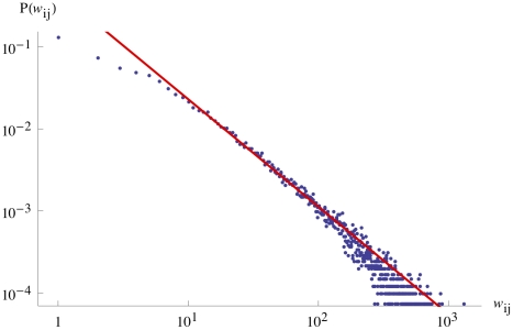
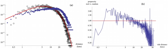
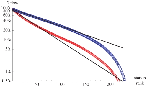
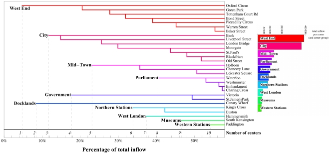
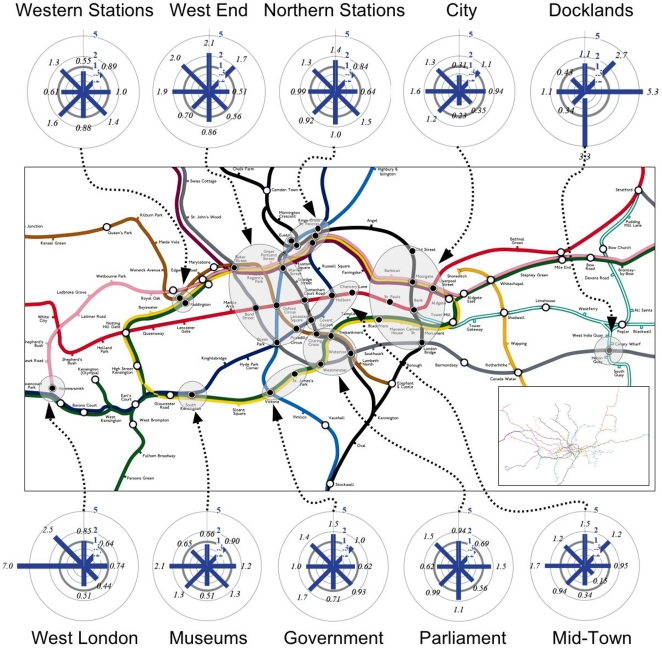
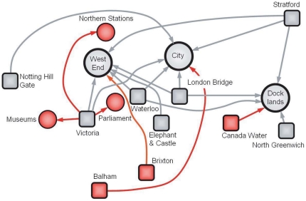
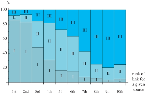
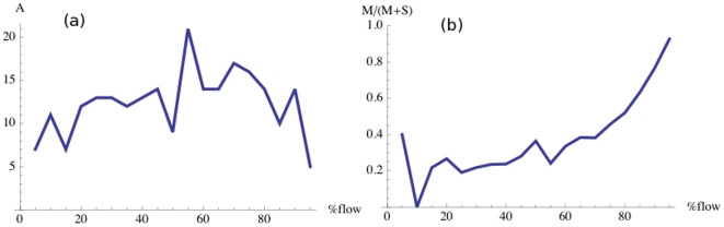
The spatial arrangement of urban hubs and centers and how individuals interact with these centers is a crucial problem with many applications ranging from urban planning to epidemiology. We utilize here in an unprecedented manner the large scale, real-time 'Oyster' card database of individual person movements in the London subway to reveal the structure and organization of the city. We show that patterns of intraurban movement are strongly heterogeneous in terms of volume, but not in terms of distance travelled, and that there is a polycentric structure composed of large flows organized around a limited number of activity centers. For smaller flows, the pattern of connections becomes richer and more complex and is not strictly hierarchical since it mixes different levels consisting of different orders of magnitude. This new understanding can shed light on the impact of new urban projects on the evolution of the polycentric configuration of a city and the dense structure of its centers and it provides an initial approach to modeling flows in an urban system.
Overview
The claims and statistics of this paper haven’t been checked yet.
Run the check — free, no account needed. It reads the open-access text and checks the sources it cites.
Integrity signals
Registry
Cites
Statistics
Figures
Verification
Claims the paper makes
The claims and statistics of this paper haven’t been checked yet.
Run the check — free, no account needed. It reads the open-access text and checks the sources it cites.
Claims other papers make about this one
Each is checked against this paper’s own text: does it say what the citing paper says it does?
The cited source says what the claim attributes to it.
In the citing paper
“For example, a dominant model of modern city form is the clustering of economic activities in urban hubs, known as polycentricity 43,209 .”
From From cognitive maps to spatial schemas (2023) · cites this paper as [43]
In the citing paper
“Recent findings indicate that a city's spatial structure is characterized by multiple subregions (such as urban zoning areas) connected via distribution networks (such as streets) 40,43,134,135 .”
From From cognitive maps to spatial schemas (2023) · cites this paper as [43]
In the citing paper
“Urban data analytics further show that industrial cities can be classified using characteristic spatial patterns and common principles, such as an organization centred around nodes of economic activity 42,43,129,177 .”
From From cognitive maps to spatial schemas (2023) · cites this paper as [43]
In the citing paper
“Given that these statistical commonalities of mobility patterns characterize the underlying structure of a city 41,43 and navigational behaviours 34,117,178,179 , they provide support for the notion of a spatial schema for an environment with key elements that can be generalized to other environments that belong to a superordinate category 159 .”
From From cognitive maps to spatial schemas (2023) · cites this paper as [43]
In the citing paper
“Studies that focus on mathematical analyses of topology have helped us gain insight into spatial patterns that characterize different types of environments 43,135,208 .”
From From cognitive maps to spatial schemas (2023) · cites this paper as [43]
In the citing paper
“The patterns of individuals' movement to and from urban hubs across cities can be collected using GIS (geographic information system) tools and phone-usage data 40,43,177,210 .”
From From cognitive maps to spatial schemas (2023) · cites this paper as [43]
Self-check
Percentages, sums and reported differences re-computed from the paper’s own numbers.
The self-check needs the paper’s full text.
Citations
Cites
The Elements of Statistical Learning
Hastie, T., Friedman, J., & Tibshirani, R. (2001) · Springer Series in Statistics · doi:10.1007/978-0-387-21606-5 · Cited by 24,162
Understanding individual human mobility patterns
González, M. C., Hidalgo, C. A., & Barabási, A.-Ĺ. (2008) · Nature · doi:10.1038/nature06958 · Cited by 6,186
The Spatial Economy: Cities, Regions, and International Trade
Fujita, M., Krugman, P., & Venables, A. J. (1999) · doi:10.7551/mitpress/6389.001.0001 · Cited by 4,788
Random graphs with arbitrary degree distributions and their applications
Newman, M. E. J., Strogatz, S. H., & Watts, D. J. (2001) · Physical review. E, Statistical physics, plasmas, fluids, and related interdisciplinary topics · doi:10.1103/physreve.64.026118 · Cited by 3,675
A critical point for random graphs with a given degree sequence
Molloy, M. S. O., & Reed, B. A. (1995) · Random Structures and Algorithms · doi:10.1002/rsa.3240060204 · Cited by 2,267
The scaling laws of human travel
Brockmann, D., Hufnagel, L., & Geisel, T. (2006) · Nature · doi:10.1038/nature04292 · Cited by 2,182
Modelling disease outbreaks in realistic urban social networks
Eubank, S., Güçlü, H., Kumar, V. S. A., MARATHE, M. V., Srinivasan, A., Toroczkai, Z., & Wang, N. (2004) · Nature · doi:10.1038/nature02541 · Cited by 2,098
Warf, B. (2010) · Encyclopedia of Geography · doi:10.4135/9781412939591.n1196 · Cited by 1,196
Anas, A., Arnott, R., & Small, K. A. (1997) · RePEc: Research Papers in Economics · Cited by 819
The Polycentric Urban Region: Towards a Research Agenda
Kloosterman, R. C., & Musterd, S. (2001) · Urban Studies · doi:10.1080/00420980120035259 · Cited by 597
Cited by
Sorted by citations
Objective Criteria for the Evaluation of Clustering Methods
Rand, W. M. (1971) · Journal of the American Statistical Association · doi:10.1080/01621459.1971.10482356 · Cited by 6,493
Alzheimer Disease Genetics Consortium (ADGC), Kunkle, B. W., The European Alzheimer’s Disease Initiative (EADI), Cohorts for Heart and Aging Research in Genomic Epidemiology Consortium (CHARGE), Genetic and Environmental Risk in AD/Defining Genetic, P. A. E. R. F. A. D. C. (., Grenier-Boley, B., Sims, R., Bis, J. C., Damotte, V., Naj, A. C., et al. (2019) · Nature Genetics · doi:10.1038/s41588-019-0358-2 · Cited by 2,946
A universal model for mobility and migration patterns
Simini, F., González, M. C., Maritan, A., & Barabási, A.-Ĺ. (2012) · Nature · doi:10.1038/nature10856 · Cited by 1,480
Human mobility: Models and applications
Barbosa, H., Barthélemy, M., Ghoshal, G., James, C. R., Lenormand, M., Louail, T., de Menezes, R. P., Ramasco, J. J., Simini, F., & Tomasini, M. (2018) · Physics Reports · doi:10.1016/j.physrep.2018.01.001 · Cited by 1,104
Self-citationKees, J., Berry, C., Burton, S., & Sheehan, K. (2017) · Journal of Advertising · doi:10.1080/00913367.2016.1269304 · Cited by 902
Social Sensing: A New Approach to Understanding Our Socioeconomic Environments
Liu, Y., Liu, X., Gao, S., Gong, L., Kang, C., Zhi, Y., Chi, G., & Shi, L. (2015) · Annals of the Association of American Geographers · doi:10.1080/00045608.2015.1018773 · Cited by 821
Detecting the dynamics of urban structure through spatial network analysis
Zhong, C., Arisona, S. M., Huang, X., Batty, M., & Schmitt, G. (2014) · International Journal of Geographical Information Systems · doi:10.1080/13658816.2014.914521 · Cited by 524
Self-citationFrom mobile phone data to the spatial structure of cities
Louail, T., Lenormand, M., Cantú-Ros, O. G., Picornell, M., Herranz, R., Frı́as, M., Ramasco, J. J., & Barthélemy, M. (2014) · Scientific Reports · doi:10.1038/srep05276 · Cited by 457
Self-citationRevealing travel patterns and city structure with taxi trip data
Liu, X., Li, G., Gong, Y., & Liu, Y. (2015) · Journal of Transport Geography · doi:10.1016/j.jtrangeo.2015.01.016 · Cited by 447
Uncovering Patterns of Inter-Urban Trip and Spatial Interaction from Social Media Check-In Data
Liu, Y., Sui, Z., Kang, C., & Gao, Y. C. (2014) · PLoS ONE · doi:10.1371/journal.pone.0086026 · Cited by 393
Spatiotemporal Patterns of Urban Human Mobility
Hasan, S., Schneider, C., Ukkusuri, S. V., & González, M. C. (2012) · Journal of Statistical Physics · doi:10.1007/s10955-012-0645-0 · Cited by 282
Who Benefits from the "Sharing" Economy of Airbnb?
Giovanni Quattrone, A., Proserpio, D., Quercia, D., Capra, L., & Musolesi, M. (2016) · International World Wide Web Conference (WWW) · doi:10.1145/2872427.2874815 · Cited by 275
Long, Y., & Thill, J. (2015) · Computers Environment and Urban Systems · doi:10.1016/j.compenvurbsys.2015.02.005 · Cited by 265
A review of urban computing for mobile phone traces
Jiang, S., Fiore, G. A., Yang, Y., Ferreira, J., Frazzoli, E., & González, M. C. (2013) · ACM SIGKDD International Workshop on Urban Computing (UrbComp) · doi:10.1145/2505821.2505828 · Cited by 251
SHARED BICYCLES IN A CITY: A SIGNAL PROCESSING AND DATA ANALYSIS PERSPECTIVE
Borgnat, P., Abry, P., Flandrin, P., Robardet, C., Rouquier, J., & Eric Fleury, B. (2011) · Advances in Complex Systems · doi:10.1142/s0219525911002950 · Cited by 252
Big Data for Social Transportation
Zheng, X., Chen, W., Wang, P., Shen, D., Chen, S., Wang, X., Zhang, Q., & Yang, L. (2015) · IEEE Transactions on Intelligent Transportation Systems · doi:10.1109/tits.2015.2480157 · Cited by 243
Revealing travel patterns and city structure with taxi trip data
Liu, X., Li, G., Gong, Y., & Liu, Y. (2015) · RePEc: Research Papers in Economics · Cited by 246
Human mobility and socioeconomic status: Analysis of Singapore and Boston
Xu, Y., Belyi, A., Bojić, I., & Ratti, C. (2018) · Computers Environment and Urban Systems · doi:10.1016/j.compenvurbsys.2018.04.001 · Cited by 235
Rethinking big data: A review on the data quality and usage issues
Liu, J., Li, J., Li, W., & Wu, J. (2015) · ISPRS Journal of Photogrammetry and Remote Sensing · doi:10.1016/j.isprsjprs.2015.11.006 · Cited by 240
How congestion shapes cities: from mobility patterns to scaling
Louf, R., & Barthélemy, M. (2014) · Scientific Reports · doi:10.1038/srep05561 · Cited by 266
Self-citationDynamical Patterns of Cattle Trade Movements
Bajardi, P., Barrat, A., Natale, F., Savini, L., & Colizza, V. (2011) · PLoS ONE · doi:10.1371/journal.pone.0019869 · Cited by 229
Mapping Cilento: using geotagged social media data to characterize tourist flows in southern Italy
Chua, A., Servillo, L., Marcheggiani, E., & Moere, A. V. (2016) · Tourism Management · doi:10.1016/j.tourman.2016.06.013 · Cited by 216
Krol, S., Macrez, R., Docagne, F., Defer, G. L., Laurent, S., Rahman, M., Hajipour, M. J., Kehoe, P. G., & Mahmoudi, M. (2012) · Chemical Reviews · doi:10.1021/cr200472g · Cited by 219
Yue, Y., Lan, T., Yeh, A. G. O., & Li, Q. (2014) · Travel Behaviour and Society · doi:10.1016/j.tbs.2013.12.002 · Cited by 216
Hierarchical organization of urban mobility and its connection with city livability
Bassolas, A., Barbosa, H., Dickinson, B., Dotiwalla, X., Eastham, P., Gallotti, R., Ghoshal, G., Gipson, B. R., Hazarie, S. A., Kautz, H., et al. (2019) · Nature Communications · doi:10.1038/s41467-019-12809-y · Cited by 214
A city of cities: Measuring how 15-minutes urban accessibility shapes human mobility in Barcelona
Graells-Garrido, E., Serra-Burriel, F., Rowe, F., Cucchietti, F., & Reyes, P. (2021) · PLoS ONE · doi:10.1371/journal.pone.0250080 · Cited by 204
Uncovering the spatial structure of mobility networks
Louail, T., Lenormand, M., Picornell, M., García Cantú, O., Herranz, R., Frias-Martinez, E., Ramasco, J. J., & Barthelemy, M. (2015) · Nature Communications · doi:10.1038/ncomms7007 · Cited by 203
Knockdown of MLO genes reduces susceptibility to powdery mildew in grapevine
Pessina, S., Lenzi, L., Perazzolli, M., Campa, M., Costa, L. D., Urso, S., Valè, G., Salamini, F., Velasco, R., & Malnoy, M. (2016) · Horticulture Research · doi:10.1038/hortres.2016.16 · Cited by 200
Universal predictability of mobility patterns in cities
Yan, X.-Y., Zhao, C., Fan, Y., Di, Z., & Wang, W.-X. (2014) · Journal of The Royal Society Interface · doi:10.1098/rsif.2014.0834 · Cited by 197
Chen, T., Hui, E. C. M., Wu, J., Lang, W., & Li, X. (2019) · Habitat International · doi:10.1016/j.habitatint.2019.102005 · Cited by 196
Mahabir, R., Croitoru, A., Crooks, A. T., Agouris, P., & Stefanidis, A. (2018) · Urban Science · doi:10.3390/urbansci2010008 · Cited by 195
Revealing centrality in the spatial structure of cities from human activity patterns
Zhong, C., Schläpfer, M., Arisona, S. M., Batty, M., Ratti, C., & Schmitt, G. (2015) · Urban Studies · doi:10.1177/0042098015601599 · Cited by 192
Self-citationAgglomerations and the rise of urban network externalities
Burger, M., & Meijers, E. J. (2016) · Papers of the Regional Science Association · doi:10.1111/pirs.12223 · Cited by 187
Chopra, S. S., Dillon, T., Bilec, M. M., & Khanna, V. (2016) · Journal of The Royal Society Interface · doi:10.1098/rsif.2016.0113 · Cited by 206
Zhong, C., Batty, M., Manley, E., Wang, J., Wang, Z., Chen, F., & Schmitt, G. (2016) · PLoS ONE · doi:10.1371/journal.pone.0149222 · Cited by 175
Self-citationPark, S., Xu, Y., Jiang, L., Chen, Z., & Huang, S. (2020) · Annals of Tourism Research · doi:10.1016/j.annals.2020.102973 · Cited by 202
Predicting commuter flows in spatial networks using a radiation model based on temporal ranges
Ren, Y., Ercsey-Ravasz, M., Wang, P., González, M. C., & Toroczkai, Z. (2014) · Nature Communications · doi:10.1038/ncomms6347 · Cited by 177
Antibacterial activity of selected Malaysian honey
Zainol, M. I. B., Yusoff, K. M., & Yusof, M. Y. M. (2013) · BMC Complementary and Alternative Medicine · doi:10.1186/1472-6882-13-129 · Cited by 177
Understanding urban mobility patterns with a probabilistic tensor factorization framework
Sun, L., & Axhausen, K. W. (2016) · Transportation Research Part B Methodological · doi:10.1016/j.trb.2016.06.011 · Cited by 175
Urban Mobility and Activity Space
Cagney, K. A., Cornwell, E. Y., Goldman, A. W., & Cai, L. (2020) · Annual Review of Sociology · doi:10.1146/annurev-soc-121919-054848 · Cited by 184
Unraveling the origin of exponential law in intra-urban human mobility
Liang, X., Zhao, J., Dong, L., & Xu, K. (2013) · Scientific Reports · doi:10.1038/srep02983 · Cited by 165
Diversity of individual mobility patterns and emergence of aggregated scaling laws
Yan, X.-Y., Han, X.-P., Wang, B.-H., & Zhou, T. (2013) · Scientific Reports · doi:10.1038/srep02678 · Cited by 160
Using mobility data as proxy for measuring urban vitality
Sulis, P., Manley, E., Zhong, C., & Batty, M. (2018) · Journal of Spatial Information Science · doi:10.5311/josis.2018.16.384 · Cited by 154
Self-citationHow congestion shapes cities: from mobility patterns to scaling.
Louf, R., & Barthelemy, M. (2014) · UCL Discovery (University College London) · Cited by 152
Modeling the Polycentric Transition of Cities
Louf, R., & Barthélemy, M. (2013) · Physical Review Letters · doi:10.1103/physrevlett.111.198702 · Cited by 146
Self-citationPolycentric urban development and urban thermal environment: A case of Hangzhou, China
Yue, W., Qiu, S., Hui, X., Xu, L., & Zhang, L. (2019) · Landscape and Urban Planning · doi:10.1016/j.landurbplan.2019.04.008 · Cited by 146
The Structure of Spatial Networks and Communities in Bicycle Sharing Systems
Austwick, M. Z., O’Brien, O., Strano, E., & Viana, M. P. (2013) · PLoS ONE · doi:10.1371/journal.pone.0074685 · Cited by 142
Evaluating the Privacy Risk of Location-Based Services
Freudiger, J., Shokri, R., & Hubaux, J. (2012) · Lecture notes in computer science · doi:10.1007/978-3-642-27576-0_3 · Cited by 145
Exploiting Foursquare and Cellular Data to Infer User Activity in Urban Environments
Noulas, A., Cecilia Mascolo, C., & Frı́as-Martı́nez, E. (2013) · IEEE International Conference on Mobile Data Management (MDM) · doi:10.1109/mdm.2013.27 · Cited by 133
Inferring building functions from a probabilistic model using public transportation data
Zhong, C., Huang, X., Arisona, S. M., Schmitt, G., & Batty, M. (2014) · Computers Environment and Urban Systems · doi:10.1016/j.compenvurbsys.2014.07.004 · Cited by 131
Self-citationA Universal Model of Commuting Networks
Lenormand, M., Huet, S., Gargiulo, F., & Deffuant, G. (2012) · PLoS ONE · doi:10.1371/journal.pone.0045985 · Cited by 128
Renaissance of protein crystallization and precipitation in biopharmaceuticals purification
dos Santos, R., Carvalho, A. L., & Roque, A. C. A. (2016) · Biotechnology Advances · doi:10.1016/j.biotechadv.2016.11.005 · Cited by 128
Understanding mobility in a social petri dish
Szell, M., Sinatra, R., Petri, G., Stefan Thurner, A., & Latora, V. (2012) · Scientific Reports · doi:10.1038/srep00457 · Cited by 116
Zhang, Y., Marshall, S., & Manley, E. (2019) · Journal of Transport Geography · doi:10.1016/j.jtrangeo.2019.102485 · Cited by 116
From cognitive maps to spatial schemas
Farzanfar, D., Spiers, H. J., Moscovitch, M., & Rosenbaum, R. S. (2023) · Nature Reviews Neuroscience · doi:10.1038/s41583-022-00655-9 · Cited by 115
A stochastic model of randomly accelerated walkers for human mobility
Gallotti, R., Bazzani, A., Rambaldi, S., & Barthélemy, M. (2016) · Nature Communications · doi:10.1038/ncomms12600 · Cited by 114
Self-citationSystematic review and meta-analysis of genetic risk factors for neuropathic pain
Veluchamy, A., Hébert, H. L., Meng, W., Palmer, C. N. A., & Smith, B. H. (2018) · Pain · doi:10.1097/j.pain.0000000000001164 · Cited by 116
Sun, Y., Fan, H., Li, M., & Zipf, A. (2015) · Environment and Planning B Planning and Design · doi:10.1177/0265813515617642 · Cited by 111
Extensive tissue-specific transcriptomic plasticity in maize primary roots upon water deficit
Opitz, N., Marcon, C., Paschold, A., Malik, W. A., Lithio, A., Brandt, R., Piepho, H., Nettleton, D. S., & Hochholdinger, F. (2015) · Journal of Experimental Botany · doi:10.1093/jxb/erv453 · Cited by 104
Saberi, M., Mahmassani, H. S., Brockmann, D., & Hosseini, A. (2016) · Transportation · doi:10.1007/s11116-016-9706-6 · Cited by 112
Quantifying the spatial homogeneity of urban road networks via graph neural networks
Xue, J., Jiang, N., Liang, S., Pang, Q., Yabe, T., Ukkusuri, S. V., & Ma, J. (2022) · Nature Machine Intelligence · doi:10.1038/s42256-022-00462-y · Cited by 113
Characterization of the MLO gene family in Rosaceae and gene expression analysis in Malus domestica
Pessina, S., Pavan, S., Catalano, D., Gallotta, A., Visser, R. G. F., Bai, Y., Malnoy, M., & Schouten, H. J. (2014) · BMC Genomics · doi:10.1186/1471-2164-15-618 · Cited by 102
Detecting Urban Polycentric Structure from POI Data
Deng, Y., Liu, J., Liu, Y., & Luo, A. (2019) · ISPRS International Journal of Geo-Information · doi:10.3390/ijgi8060283 · Cited by 102
Gan, Z., Yang, M., Feng, T., & Timmermans, H. J. P. (2018) · Transportation · doi:10.1007/s11116-018-9885-4 · Cited by 99
Improving the accessibility of urban transportation networks for people with disabilities
Ferrari, L., Berlingerio, M., Calabrese, F., & Reades, J. (2013) · Transportation Research Part C Emerging Technologies · doi:10.1016/j.trc.2013.10.005 · Cited by 98
Predicting traffic volumes and estimating the effects of shocks in massive transportation systems
Silva, R., Kang, S. M., & Airoldi, E. M. (2015) · Proceedings of the National Academy of Sciences · doi:10.1073/pnas.1412908112 · Cited by 98
Self-citationFernández-Fueyo, E., Castanera, R., Ruiz-Dueñas, F. J., López-Lucendo, M. F., Ramírez, L., Pisabarro, A. G., & Martínez, A. T. (2014) · Fungal Genetics and Biology · doi:10.1016/j.fgb.2014.02.003 · Cited by 97
Analysis on spatiotemporal urban mobility based on online car-hailing data
Zhang, B., Chen, S., Ma, Y., Li, T., & Tang, K. (2019) · Journal of Transport Geography · doi:10.1016/j.jtrangeo.2019.102568 · Cited by 97
Schiller, L., Alava, J. J., Grove, J. S., Reck, G. K., & Pauly, D. F. (2014) · Aquatic Conservation Marine and Freshwater Ecosystems · doi:10.1002/aqc.2458 · Cited by 94
Yan, X., Sedykh, A., Wang, W., Zhao, X., Yan, B., & Zhu, H. (2019) · Nanoscale · doi:10.1039/c9nr00844f · Cited by 95
Comparing and modelling land use organization in cities
Lenormand, M., Picornell, M., Cantú-Ros, O. G., Louail, T., Herranz, R., Barthélemy, M., Frı́as, M., Miguel, M. S., & Ramasco, J. J. (2015) · Royal Society Open Science · doi:10.1098/rsos.150449 · Cited by 98
Self-citationRational Design to Improve Protein Thermostability: Recent Advances and Prospects
Yang, H., Liu, L., Li, J., Chen, J., & Du, G. (2015) · ChemBioEng Reviews · doi:10.1002/cben.201400032 · Cited by 93
Pelosi, C., Tinè, M. R., & Wurm, F. R. (2020) · European Polymer Journal · doi:10.1016/j.eurpolymj.2020.110079 · Cited by 93
Modification of the gravity model and application to the metropolitan Seoul subway system
Goh, S., Lee, K., Park, J. S., & Choi, M. Y. (2012) · Physical Review E · doi:10.1103/physreve.86.026102 · Cited by 92
Morphology of travel routes and the organization of cities
Lee, M., Barbosa, H., Youn, H., Holme, P., & Ghoshal, G. (2017) · Nature Communications · doi:10.1038/s41467-017-02374-7 · Cited by 88
Multi-scale spatio-temporal analysis of human mobility
Alessandretti, L., Sapieżyński, P., Lehmann, S., & Baronchelli, A. (2017) · PLoS ONE · doi:10.1371/journal.pone.0171686 · Cited by 87
Sobolevsky, S. L., Bojić, I., Belyi, A., Sitko, I., Hawelka, B., Arias, J. M., & Ratti, C. (2015) · IEEE International Congress on Big Data (BigData Congress) · doi:10.1109/bigdatacongress.2015.92 · Cited by 81
Ranking Station Importance With Human Mobility Patterns Using Subway Network Datasets
Xia, F., Wang, J., Kong, X., Zhang, D., & Wang, Z. (2019) · IEEE Transactions on Intelligent Transportation Systems · doi:10.1109/tits.2019.2920962 · Cited by 82
Reconstructing commuters network using machine learning and urban indicators
Spadon, G., de Carvalho, A. C. P. L. F., Rodrigues-Jr, J. F., & Alves, L. G. A. (2019) · Scientific Reports · doi:10.1038/s41598-019-48295-x · Cited by 79
Road network circuity in metropolitan areas
Giacomin, D. J., & Levinson, D. M. (2015) · Environment and Planning B Planning and Design · doi:10.1068/b130131p · Cited by 81
Predicting human mobility through the assimilation of social media traces into mobility models
Beiró, M. G., Panisson, A., Tizzoni, M., & Cattuto, C. (2016) · EPJ Data Science · doi:10.1140/epjds/s13688-016-0092-2 · Cited by 80
Zhang, S., Yang, Y., Zhen, F., Lobsang, T., & Li, Z. (2020) · Journal of Transport Geography · doi:10.1016/j.jtrangeo.2020.102938 · Cited by 79
Copy number variation detection using next generation sequencing read counts
Wang, H., Nettleton, D. S., & Ying, K. (2014) · BMC Bioinformatics · doi:10.1186/1471-2105-15-109 · Cited by 77
Lathia, N., & Capra, L. (2011) · ACM International Joint Conference on Pervasive and Ubiquitous Computing (UbiComp) · doi:10.1145/2030112.2030152 · Cited by 74
Lathia, N., Smith-Clarke, C., Froehlich, J. E., & Capra, L. (2012) · Pervasive and Mobile Computing · doi:10.1016/j.pmcj.2012.10.007 · Cited by 73
A universal opportunity model for human mobility
Liu, E., & Yan, X.-Y. (2020) · Scientific Reports · doi:10.1038/s41598-020-61613-y · Cited by 78
Understanding taxi travel patterns
Cai, H., Zhan, X., Zhu, J., Jia, X., Chiu, A. S. F., & Xu, M. (2016) · Physica A Statistical Mechanics and its Applications · doi:10.1016/j.physa.2016.03.047 · Cited by 72
Zhou, Y., Fang, Z., Thill, J., Li, Q., & Li, Y. (2015) · Computers Environment and Urban Systems · doi:10.1016/j.compenvurbsys.2015.03.001 · Cited by 71
Hayfron-Benjamin, A., Obiri‐Yeboah, D., Ayisi-Addo, S., Siakwa, M., & Mupepi, S. C. (2018) · BMC Pediatrics · doi:10.1186/s12887-018-1330-5 · Cited by 69
Spatial structure and productivity in European regions
Ouwehand, W. M., Oort, F. G. V., & Cortinovis, N. (2021) · Regional Studies · doi:10.1080/00343404.2021.1950912 · Cited by 66
Cats, O., Wang, Q., & Zhao, Y. (2015) · Journal of Transport Geography · doi:10.1016/j.jtrangeo.2015.08.005 · Cited by 66
Cao, J., Li, Q., Tu, W., Gao, Q., Cao, R., & Zhong, C. (2021) · Cities · doi:10.1016/j.cities.2020.103077 · Cited by 67
Zhang, F., Li, Z., Li, N., & Fang, D. (2019) · Sustainable Cities and Society · doi:10.1016/j.scs.2019.101671 · Cited by 64
Kong, X., Liu, Y., Wang, Y., Tong, D., & Zhang, J. (2017) · ISPRS International Journal of Geo-Information · doi:10.3390/ijgi6020038 · Cited by 64
Mining mobility data to minimise travellers' spending on public transport
Lathia, N., & Capra, L. (2011) · ACM SIGKDD Conference on Knowledge Discovery and Data Mining (KDD) · doi:10.1145/2020408.2020590 · Cited by 63
Identifying human mobility patterns using smart card data
Cats, O. (2023) · Transport Reviews · doi:10.1080/01441647.2023.2251688 · Cited by 61
Velocity-enhanced cooperation of moving agents playing public goods games
Cardillo, A., Meloni, S., Gómez‐Gardeñes, J., & Moreno, Y. (2012) · Physical Review E · doi:10.1103/physreve.85.067101 · Cited by 61
Distribution, abundance and habitat use of deep diving cetaceans in the North-East Atlantic
Rogan, E., Cañadas, A., Macleod, K., Santos, M. B., Mikkelsen, B., Uriarte, A., Canneyt, O. V., Vázquez, J. A., & Hammond, P. S. (2017) · Deep Sea Research Part II Topical Studies in Oceanography · doi:10.1016/j.dsr2.2017.03.015 · Cited by 60
Yu, W. (2018) · IEEE Transactions on Intelligent Transportation Systems · doi:10.1109/tits.2018.2834573 · Cited by 60
Schwanen, T. (2016) · Progress in Human Geography · doi:10.1177/0309132516628259 · Cited by 62
Metadata
- Authors
- Roth, C., Kang, S. M., Batty, M., & Barthélemy, M.
- Affiliations
- Centre National de la Recherche Scientifique (FR)
- University College London (GB)
- Corresponding author
- Barthélemy, Marc
- Venue
- PLoS ONE
- Publisher
- Public Library of Science (PLoS)
- Published
- 2011-01-07
- Volume
- 6
- Issue
- 1
- Pages
- e15923
- ISSN
- 1932-6203 (ISSN-L)
- PMC
- PMC3017563
- OpenAlex
- W2015480405
- Cited by
- 461
- References
- 31
- Citations by year
- 2026: 10 · 2025: 19 · 2024: 14 · 2023: 19 · 2022: 25 · 2021: 36 · 2020: 43 · 2019: 48 · 2018: 39 · 2017: 39 · 2016: 50 · 2015: 39 · 2014: 31 · 2013: 22 · 2012: 19
- FWCI
- 72.59
- Type
- journal article
- Language
- en
- Open access
- gold
- doi.org
- Locations
- PLoS ONE (publishedVersion, cc-by)
- PubMed Central (publishedVersion, cc-by)
- PubMed (publishedVersion)
- arXiv (Cornell University) (submittedVersion)
- RePEc: Research Papers in Economics (submittedVersion)
- DOAJ (DOAJ: Directory of Open Access Journals) (submittedVersion)
- UCL Discovery (University College London) (submittedVersion)
- arXiv (Cornell University)
- Topics
- Social Sciences › Transportation › Human Mobility and Location-Based Analysis
- Social Sciences › Urban Studies › Urban Design and Spatial Analysis
- Social Sciences › Urban Studies › Global Urban Networks and Dynamics
- Keywords
- urban mobility, activity centers, flow heterogeneity, urban hubs
- MeSH terms
- City Planning, Humans, London, Population Dynamics, Urban Population
About these checks
Registry, retraction, Cites and statistics results are computed, not judged, with one exception: a printed reference that no index lists is read once by a model before it counts as a citation error. Claims are extracted by a model and kept only when their quote appears verbatim in the text; each cited source is then checked, with a model’s help, for whether it says what the claim relies on. Those verdicts can be wrong — read the claim’s quote and the cited source before relying on one.
Statistics and arithmetic are recomputed, not judged.
Confidence bands are shown only for fields calibrated on our annotated test set. None is calibrated yet, so no band is shown.
What counts as a claim ›How we measure confidence ›How we check this ›
Are you an author, or do you see a problem with this page? Request a review
