

The DOI matches its Crossref record; 65 of the 65 references it cites were found in a registry or an index.
An efficient quantum algorithm for the time evolution of parameterized circuits
Open accessAbstract
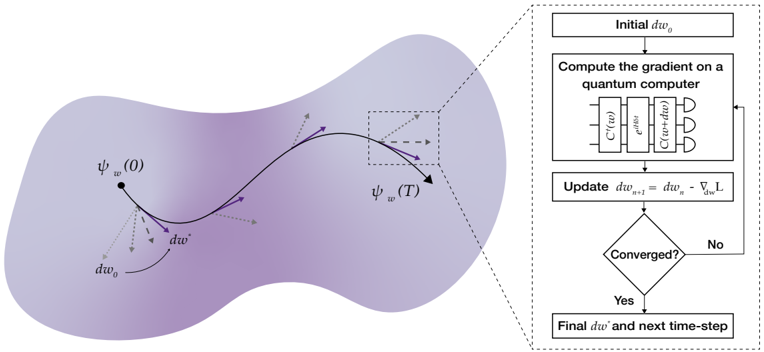
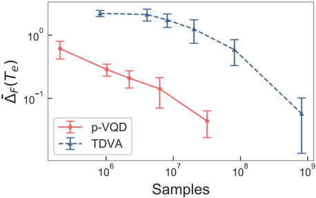
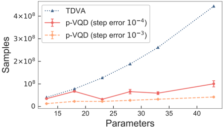
We introduce a novel hybrid algorithm to simulate the real-time evolution of quantum systems using parameterized quantum circuits. The method, named "projected – Variational Quantum Dynamics" (p-VQD) realizes an iterative, global projection of the exact time evolution onto the parameterized manifold. In the small time-step limit, this is equivalent to the McLachlan's variational principle. Our approach is efficient in the sense that it exhibits an optimal linear scaling with the total number of variational parameters. Furthermore, it is global in the sense that it uses the variational principle to optimize all parameters at once. The global nature of our approach then significantly extends the scope of existing efficient variational methods, that instead typically rely on the iterative optimization of a restricted subset of variational parameters. Through numerical experiments, we also show that our approach is particularly advantageous over existing global optimization algorithms based on the time-dependent variational principle that, due to a demanding quadratic scaling with parameter numbers, are unsuitable for large parameterized quantum circuits.
Overview
The claims and statistics of this paper haven’t been checked yet.
Free: it reads the open-access text and checks the first 5 claims that cite a source we can check. Create a free account to check every claim.
Integrity signals
Registry
Cites
Statistics
Figures
Verification
Claims the paper makes
The claims and statistics of this paper haven’t been checked yet.
Free: it reads the open-access text and checks the first 5 claims that cite a source we can check. Create a free account to check every claim.
Claims other papers make about this one
Each is checked against this paper’s own text: does it say what the citing paper says it does?
The cited source says what the claim attributes to it.
In the citing paper
“If one wants to avoid optimizing with respect to a projector onto a single state, one can instead use a local observable that also becomes maximal for the target state, namely ˆ O = 1 N ∑ N k = 1 ∣ 0 k ⟩ ⟨ 0 k ∣ ⊗ I ¯ k , where I ¯ k is the identity matrix for all qubits except k and ∣ 0 k ⟩ is the zero state for qubit k (Barison et al. , 2021; Cerezo et al. , 2021).”
From Noisy intermediate-scale quantum algorithms (2022) · cites this paper as Barison et al., 2021
The cited source says what the claim attributes to it.
In the citing paper
“Alternatively, the projected - Variational Quantum Dynamics method (p-VQD) has been proposed to bypass the measurement of aforementioned matrices (Barison et al. , 2021; Otten et al. , 2019).”
From Noisy intermediate-scale quantum algorithms (2022) · cites this paper as Barison et al. , 2021
Self-check
Percentages, sums and reported differences re-computed from the paper’s own numbers.
The self-check needs the paper’s full text.
Citations
Cites
Algorithms for quantum computation: discrete logarithms and factoring
Shor, P. W. (2002) · Proceedings 35th Annual Symposium on Foundations of Computer Science · doi:10.1109/sfcs.1994.365700 · Cited by 8,713
Quantum supremacy using a programmable superconducting processor
Arute, F., Arya, K., Babbush, R., Bacon, D., Bardin, J. C., Barends, R., Biswas, R., Boixo, S., Brandao, F. G. S. L., Buell, D. A., et al. (2019) · Nature · doi:10.1038/s41586-019-1666-5 · Cited by 7,720
Biamonte, J., Wittek, P., Pancotti, N., Rebentrost, P., Wiebe, N., & Lloyd, S. (2017) · Nature · doi:10.1038/nature23474 · Cited by 4,779
A variational eigenvalue solver on a photonic quantum processor
Peruzzo, A., McClean, J., Shadbolt, P., Yung, M.-H., Zhou, X.-Q., Love, P. J., Aspuru-Guzik, A., & O’Brien, J. L. (2014) · Nature Communications · doi:10.1038/ncomms5213 · Cited by 4,552 · cited 1×
“To circumvent the problem, current generations of quantum algorithms rely on a hybrid classicalquantum approach [8, 9, 10, 11, 12, 13].”
MethodVariational quantum algorithms
Cerezo, M., Arrasmith, A., Babbush, R., Benjamin, S. C., Endo, S., Fujii, K., McClean, J. R., Mitarai, K., Yuan, X., Cincio, L., et al. (2021) · Nature Reviews Physics · doi:10.1038/s42254-021-00348-9 · Cited by 3,385 · cited 1×
“To circumvent the problem, current generations of quantum algorithms rely on a hybrid classicalquantum approach [8, 9, 10, 11, 12, 13].”
MethodNote on Exchange Phenomena in the Thomas Atom
Dirac, P. A. M. (1930) · Mathematical Proceedings of the Cambridge Philosophical Society · doi:10.1017/s0305004100016108 · Cited by 3,302
Hardware-efficient variational quantum eigensolver for small molecules and quantum magnets
Kandala, A., Mezzacapo, A., Temme, K., Takita, M., Brink, M., Chow, J. M., & Gambetta, J. M. (2017) · Nature · doi:10.1038/nature23879 · Cited by 2,982
Georgescu, I. M., Ashhab, S., & Nori, F. (2014) · Reviews of Modern Physics · doi:10.1103/revmodphys.86.153 · Cited by 2,932
Supervised learning with quantum-enhanced feature spaces
Havlíček, V., Córcoles, A. D., Temme, K., Harrow, A. W., Kandala, A., Chow, J. M., & Gambetta, J. M. (2019) · Nature · doi:10.1038/s41586-019-0980-2 · Cited by 2,572
Barren plateaus in quantum neural network training landscapes
McClean, J. R., Boixo, S., Smelyanskiy, V. N., Babbush, R., & Neven, H. (2018) · Nature Communications · doi:10.1038/s41467-018-07090-4 · Cited by 2,329
Research works printed but not linked: 2
- Iordanis Kerenidis, Jonas Landman, Alessandro Luongo, and Anupam Prakash, ``q-means: A quantum algorithm for unsupervised machine learning'' Advances in Neural Information Processing Systems 32, 4134–4144 (2019).
- Jacov Frenkel ``Wave Mechanics: Advanced General Theory'' Oxford University Press (1934).
Cited by
Noisy intermediate-scale quantum algorithms
Bharti, K., Cervera-Lierta, A., Kyaw, T. H., Haug, T., Alperin-Lea, S., Anand, A., Degroote, M., Heimonen, H., Kottmann, J. S., Menke, T., et al. (2022) · Reviews of Modern Physics · doi:10.1103/revmodphys.94.015004 · Cited by 2,231
Quantum Computing for High-Energy Physics: State of the Art and Challenges
Di Meglio, A., Jansen, K., Tavernelli, I., Alexandrou, C., Arunachalam, S., Bauer, C. W., Borras, K., Carrazza, S., Crippa, A., Croft, V., et al. (2024) · PRX Quantum · doi:10.1103/prxquantum.5.037001 · Cited by 215
The future of quantum computing with superconducting qubits
Bravyi, S., Dial, O., Gambetta, J. M., Gil, D., & Nazario, Z. (2022) · Journal of Applied Physics · doi:10.1063/5.0082975 · Cited by 334
Emerging quantum computing algorithms for quantum chemistry
Motta, M., & Rice, J. E. (2022) · WIREs Computational Molecular Science · doi:10.1002/wcms.1580 · Cited by 173
NISQ computing: where are we and where do we go?
Lau, J. W. Z., Lim, K. H., Shrotriya, H., & Kwek, L. C. (2022) · AAPPS Bulletin · doi:10.1007/s43673-022-00058-z · Cited by 173
Metadata
- Authors
- Barison, S., Vicentini, F., & Carleo, G.
- Affiliations
- École Polytechnique Fédérale de Lausanne (CH)
- Venue
- Quantum
- Published
- 2021-07-28
- Volume
- 5
- Pages
- 512
- ISSN
- 2521-327X (ISSN-L)
- OpenAlex
- W3120410077
- Cited by
- 110
- References
- 58
- Citations by year
- 2026: 6 · 2025: 19 · 2024: 24 · 2023: 30 · 2022: 21 · 2021: 10
- FWCI
- 7.51
- Type
- journal article
- Language
- en
- Open access
- gold
- doi.org
- Locations
- Quantum (publishedVersion, cc-by)
- arXiv (Cornell University) (submittedVersion)
- DOAJ (DOAJ: Directory of Open Access Journals) (submittedVersion, cc-by-sa)
- Infoscience (Ecole Polytechnique Fédérale de Lausanne) (submittedVersion, cc-by-nc-nd)
- arXiv (Cornell University) (cc-by)
- Topics
- Physical Sciences › Computer Science › Artificial Intelligence › Quantum Computing Algorithms and Architecture
- Physical Sciences › Physics and Astronomy › Atomic and Molecular Physics, and Optics › Quantum many-body systems
- Physical Sciences › Mathematics › Numerical Analysis › Numerical Solvers for Ordinary Differential Equations
- Keywords
- variational quantum circuits, time-dependent variational principle, hybrid quantum-classical algorithms
About these checks
Registry, retraction, Cites and statistics results are computed, not judged, with one exception: a printed reference that no index lists is read once by a model before it counts as a citation error. Claims are extracted by a model and kept only when their quote appears verbatim in the text; each cited source is then checked, with a model’s help, for whether it says what the claim relies on. Those verdicts can be wrong — read the claim’s quote and the cited source before relying on one.
Statistics and arithmetic are recomputed, not judged.
Confidence bands are shown only for fields calibrated on our annotated test set. None is calibrated yet, so no band is shown.
What counts as a claim ›How we measure confidence ›How we check this ›
Are you an author, or do you see a problem with this page? Request a review
How to cite
Cite CoChat for the checks on this page, and the paper for its own findings.
- This page
- CoChat. (2026). Citation check: An efficient quantum algorithm for the time evolution of parameterized circuits. https://app.cochat.ai/papers/10.22331/q-2021-07-28-512
- The paper
- Barison, S., Vicentini, F., & Carleo, G. (2021). An efficient quantum algorithm for the time evolution of parameterized circuits. Quantum. https://doi.org/10.22331/q-2021-07-28-512
Data sources
Bibliographic data: Semantic Scholar, OpenAlex, Crossref.
Contains information from the Semantic Scholar Academic Graph Datasets, made available under the ODC Attribution License (ODC-BY 1.0).
Semantic Scholar’s data is described in: Kinney, R., et al. (2023). The Semantic Scholar Open Data Platform. arXiv:2301.10140.
