Cited by 9

The DOI matches its Crossref record; 1 of the 1 references it cites were found in a registry or an index.

Feedback mechanisms and sensitivities of ocean carbon uptake under global warming

Plattner, G.-K., Joos, F., Stocker, T. F., Marchal, O.·2001·Tellus B: Chemical and Physical Meteorology

Overview

The claims and statistics of this paper haven’t been checked yet.

Run the check — free, no account needed. It reads the open-access text and checks the sources it cites.

A few free checks a day · papers already verified open instantly · results are public

Integrity signals

Registry

Crossref · 10.3402/tellusb.v53i5.16637

Cites

1 of 1 references verified0 citation errors · 0 not checkable

Statistics

Figures

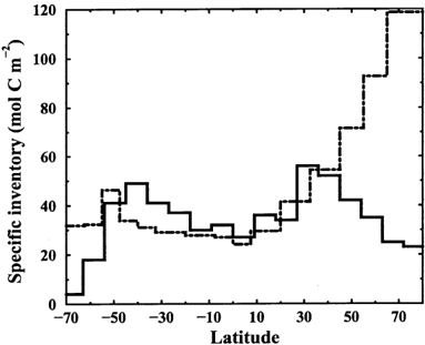
Fig. 1 Specific inventory of anthropogenic CO 2 in the Atlantic Ocean according to the data-based estimates of Gruber (1998) (solid) and the model estimates from the standard model simulation ( D T 2x = 3.7 ° C) (dot-dashed). North of the equator inventories are given for 1982; south of the equator they are given for 1989.
Fig. 1 Specific inventory of anthropogenic CO 2 in the Atlantic Ocean according to the data-based estimates of Gruber (1998) (solid) and the model estimates from the standard model simulation ( D T 2x = 3.7 ° C) (dot-dashed). North of the equator inventories are given for 1982; south of the equator they are given for 1989.CC-BY · From the PDF
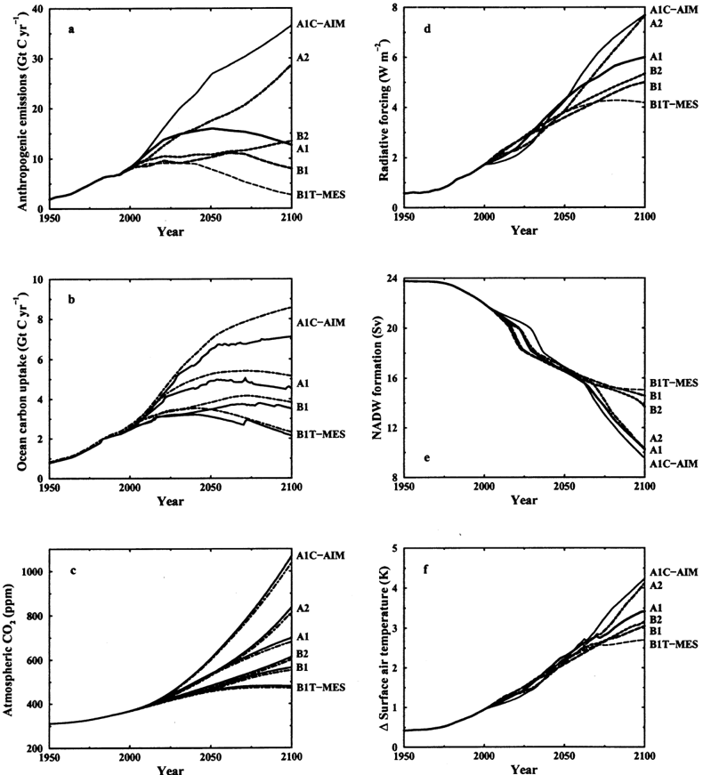
Image 2
CC-BY · From the PDF
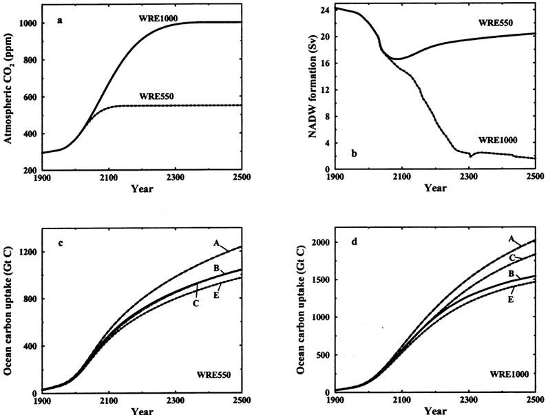
Image 3
CC-BY · From the PDF
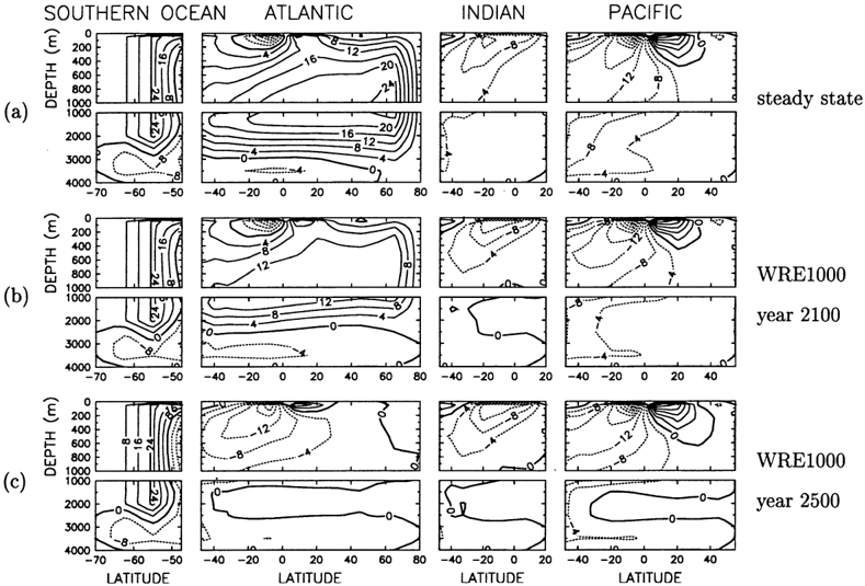
Fig. 4 Meridional overturning streamfunction (Sv) in the Southern Ocean and in the Atlantic, Indian and Pacific basins at di V erent times. (a) Preindustrial steady state (year 1765), (b) year 2100 and (c) year 2500 for CO 2 stabilization profile WRE1000. Results in (b) and (c) are produced with the standard model setup ( D T 2x = 3.7 ° C). Contour interval is 8 Sv in the Southern Ocean and 4 Sv in the Atlantic, Indian and Pacific basins.
Fig. 4 Meridional overturning streamfunction (Sv) in the Southern Ocean and in the Atlantic, Indian and Pacific basins at di V erent times. (a) Preindustrial steady state (year 1765), (b) year 2100 and (c) year 2500 for CO 2 stabilization profile WRE1000. Results in (b) and (c) are produced with the standard model setup ( D T 2x = 3.7 ° C). Contour interval is 8 Sv in the Southern Ocean and 4 Sv in the Atlantic, Indian and Pacific basins.CC-BY · From the PDF
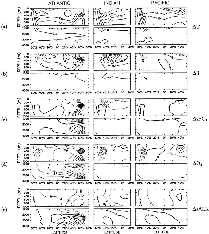
Fig. 5 Latitude-depth distribution of changes in physical and biogeochemical properties in the three main oceanic basins at year 2100 relative to the preindustrial steaty state. (a) Ocean temperature (K), (b) ocean salinity (psu), (c) salinity-normalized PO 4 (sPO 4 in mmol m -3 ), (d) O 2 (mmol m -3 ) and (e) salinity-normalized ALK (sALK in meq m -3 ). Results are shown for the standard model setup ( D T 2x = 3.7 ° C) and CO 2 stabilization scenario WRE1000. Contour intervals in (d) and (e) are unequally spaced for clarity. Contour intervals and applied ranges are as follows: (a) 0.5 ° C from -1 to + 3.5, (b) 0.1 psu from -0.5 to + 0.8, (c) 0.1 mmol m -3 from -0.6 to + 0.7, (d) 20 mmol m -3 from -170 to -50 and 10 mmol m -3 from -50 to + 30, and (e) 5 meq m -3 from -30 to + 10 and 10 meq m -3 from + 10 to + 80.
Fig. 5 Latitude-depth distribution of changes in physical and biogeochemical properties in the three main oceanic basins at year 2100 relative to the preindustrial steaty state. (a) Ocean temperature (K), (b) ocean salinity (psu), (c) salinity-normalized PO 4 (sPO 4 in mmol m -3 ), (d) O 2 (mmol m -3 ) and (e) salinity-normalized ALK (sALK in meq m -3 ). Results are shown for the standard model setup ( D T 2x = 3.7 ° C) and CO 2 stabilization scenario WRE1000. Contour intervals in (d) and (e) are unequally spaced for clarity. Contour intervals and applied ranges are as follows: (a) 0.5 ° C from -1 to + 3.5, (b) 0.1 psu from -0.5 to + 0.8, (c) 0.1 mmol m -3 from -0.6 to + 0.7, (d) 20 mmol m -3 from -170 to -50 and 10 mmol m -3 from -50 to + 30, and (e) 5 meq m -3 from -30 to + 10 and 10 meq m -3 from + 10 to + 80.CC-BY · From the PDF
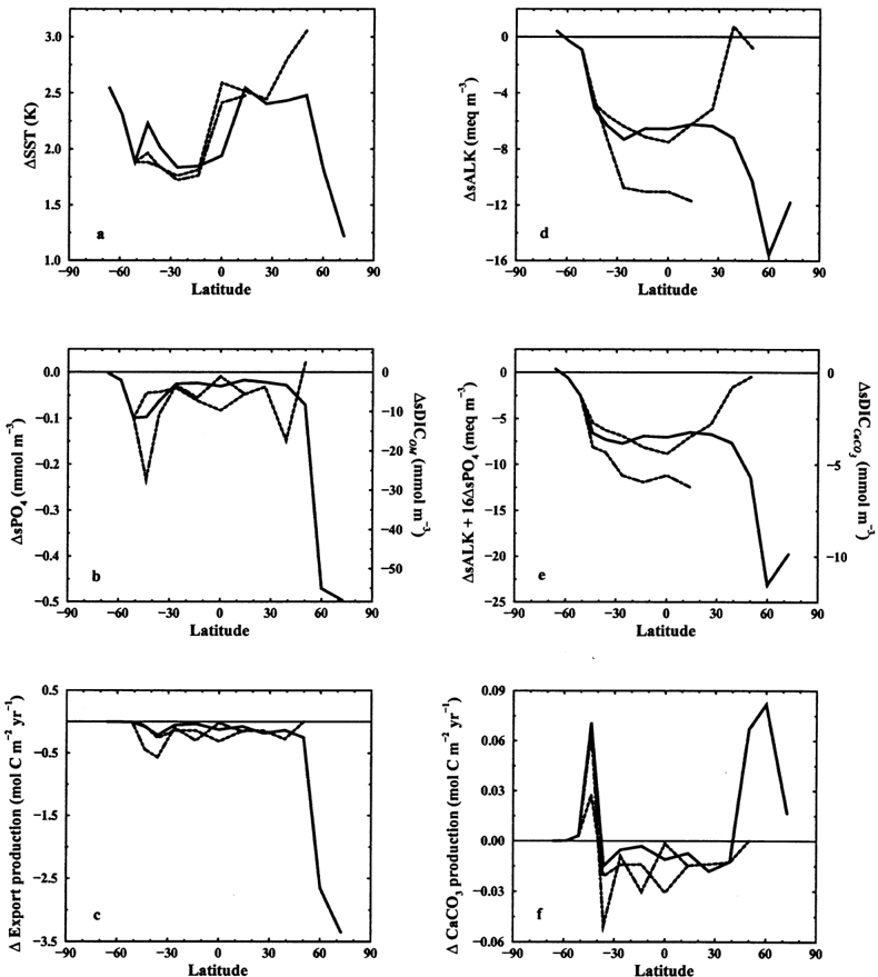
Fig. 6 Latitudinal distribution of changes in (a) sea-surface temperatures, (b) salinity-normalized euphotic zone PO 4 , sPO 4 , (c) export production of organic matter (OM), (d) salinity-normalized euphotic zone ALK, sALK, (e) salinitynormalized euphotic zone ALK from changes in the CaCO 3 cycle, and (f ) CaCO 3 production in the three main oceanic basins until year 2100. Results are shown for the standard model setup ( D T 2x = 3.7 ° C) and stabilization scenario WRE1000. The di V erent curves classify the Atlantic (solid), Indian (dot-dashed) and Pacific (dashed) basins. In panels (c) and (d) the right axis indicates the range of related changes in salinity-normalized DIC due to the internal reorganization of the OM cycle, D sDIC OM , and due to the internal reorganization of the CaCO 3 cycle, D sDIC CaCO 3 .
Fig. 6 Latitudinal distribution of changes in (a) sea-surface temperatures, (b) salinity-normalized euphotic zone PO 4 , sPO 4 , (c) export production of organic matter (OM), (d) salinity-normalized euphotic zone ALK, sALK, (e) salinitynormalized euphotic zone ALK from changes in the CaCO 3 cycle, and (f ) CaCO 3 production in the three main oceanic basins until year 2100. Results are shown for the standard model setup ( D T 2x = 3.7 ° C) and stabilization scenario WRE1000. The di V erent curves classify the Atlantic (solid), Indian (dot-dashed) and Pacific (dashed) basins. In panels (c) and (d) the right axis indicates the range of related changes in salinity-normalized DIC due to the internal reorganization of the OM cycle, D sDIC OM , and due to the internal reorganization of the CaCO 3 cycle, D sDIC CaCO 3 .CC-BY · From the PDF
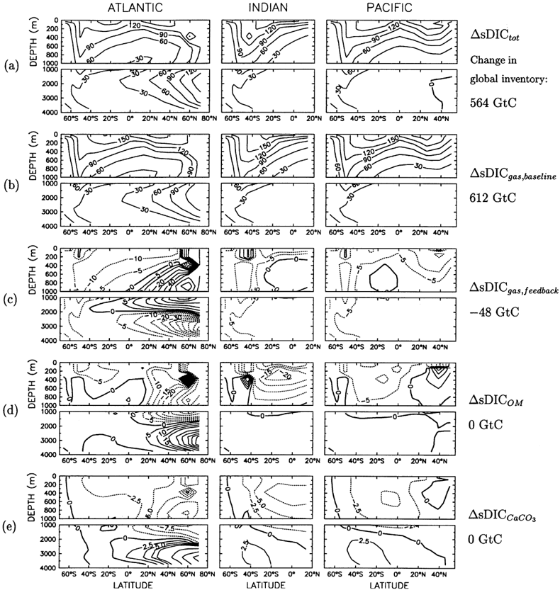
Fig. 7 Latitude-depth distribution of changes in salinity-normalized DIC (sDIC) in the three main oceanic basins until year 2100. (a) Total change in sDIC ( D sDIC tot in mmol m -3 ) from the standard model setup ( D T 2x = 3.7 ° C), ( b) excess sDIC due to gas exchange only ( D sDIC gas,baseline in mmol m -3 ) from the constant-climate baseline simulation ( D T 2x = 0 ° C) compared to the preindustrial steady state, (c) D sDIC due to the changes in air-sea gas exchange ( D sDIC gas,feedback in mmol m -3 ), (d) D sDIC due to the internal reorganisation of the OM cycle ( D sDIC OM in mmol m -3 ), and (e) D sDIC due to the internal reorganisation of the CaCO 3 cycle ( D sDIC CaCO 3 in mmol m -3 ) at year 2100 from the standard model setup ( D T 2x = 3.7 ° C) compared to the constant-climate baseline simulation ( D T 2x = 0 ° C). All the results given are for the CO 2 stabilization profile WRE1000. sDIC inventory changes (GtC) are indicated to the right of the panels. Contour intervals in (c), (d) and (e) are unequally spaced for clarity. Contour intervals and applied ranges are as follows: (a) and (b) 30 mmol m -3 from 0 to + 190, (c) 10 mmol m -3 from -100 to -10, 5 mmol m -3 from -10 to + 10 and 10 mmol m -3 from + 10 to + 80, (d) 10 mmol m -3 from -90 to -20, 5 mmol m -3 from -20 to + 20 and 10 mmol m -3 from + 20 to + 90, and (e) 2.5 mmol m -3 from -20 to + 10 and 10 mmol m -3 from + 10 to + 50.
Fig. 7 Latitude-depth distribution of changes in salinity-normalized DIC (sDIC) in the three main oceanic basins until year 2100. (a) Total change in sDIC ( D sDIC tot in mmol m -3 ) from the standard model setup ( D T 2x = 3.7 ° C), ( b) excess sDIC due to gas exchange only ( D sDIC gas,baseline in mmol m -3 ) from the constant-climate baseline simulation ( D T 2x = 0 ° C) compared to the preindustrial steady state, (c) D sDIC due to the changes in air-sea gas exchange ( D sDIC gas,feedback in mmol m -3 ), (d) D sDIC due to the internal reorganisation of the OM cycle ( D sDIC OM in mmol m -3 ), and (e) D sDIC due to the internal reorganisation of the CaCO 3 cycle ( D sDIC CaCO 3 in mmol m -3 ) at year 2100 from the standard model setup ( D T 2x = 3.7 ° C) compared to the constant-climate baseline simulation ( D T 2x = 0 ° C). All the results given are for the CO 2 stabilization profile WRE1000. sDIC inventory changes (GtC) are indicated to the right of the panels. Contour intervals in (c), (d) and (e) are unequally spaced for clarity. Contour intervals and applied ranges are as follows: (a) and (b) 30 mmol m -3 from 0 to + 190, (c) 10 mmol m -3 from -100 to -10, 5 mmol m -3 from -10 to + 10 and 10 mmol m -3 from + 10 to + 80, (d) 10 mmol m -3 from -90 to -20, 5 mmol m -3 from -20 to + 20 and 10 mmol m -3 from + 20 to + 90, and (e) 2.5 mmol m -3 from -20 to + 10 and 10 mmol m -3 from + 10 to + 50.CC-BY · From the PDF
Image 8
CC-BY · From the PDF
Image 9
CC-BY · From the PDF
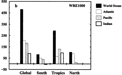
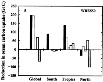
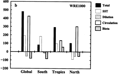
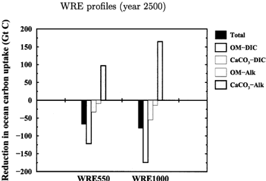
Fig. 9 Reduction in oceanic carbon uptake due to specified global warming feedbacks until year 2500. The total reduction is given for the standard model setup ( D T 2x = 3.7 ° C) and stabilization profiles WRE550 (a) and WRE1000 ( b) compared to the constant-climate baseline ( D T 2x = 0 ° C). The contributions by di V erent feedbacks are determined as described in Table 2 and listed in Table 3 (simulations A to H). Results are shown for di V erent latitudinal regions (South: 70 ° S-32.5 ° S; Tropics: 32.5 ° S-32.5 ° N; North: 32.5 ° N-80 ° N). Positive values stand for a reduction and negative values for an increase in ocean CO 2 uptake.
Fig. 9 Reduction in oceanic carbon uptake due to specified global warming feedbacks until year 2500. The total reduction is given for the standard model setup ( D T 2x = 3.7 ° C) and stabilization profiles WRE550 (a) and WRE1000 ( b) compared to the constant-climate baseline ( D T 2x = 0 ° C). The contributions by di V erent feedbacks are determined as described in Table 2 and listed in Table 3 (simulations A to H). Results are shown for di V erent latitudinal regions (South: 70 ° S-32.5 ° S; Tropics: 32.5 ° S-32.5 ° N; North: 32.5 ° N-80 ° N). Positive values stand for a reduction and negative values for an increase in ocean CO 2 uptake.CC-BY · From the PDF
Image 11
CC-BY · From the PDF

Verification

Claims the paper makes

The claims and statistics of this paper haven’t been checked yet.

Run the check — free, no account needed. It reads the open-access text and checks the sources it cites.

A few free checks a day · papers already verified open instantly · results are public

Self-check

Percentages, sums and reported differences re-computed from the paper’s own numbers.

The self-check needs the paper’s full text.

Citations

Cites

  • Simulated response of the ocean carbon cycle to anthropogenic climate warming

    Sarmiento, J. L., Hughes, T. M. C., Stouffer, R. J., & Manabe, S. (1998) · Nature · doi:10.1038/30455 · Cited by 899 · cited 10×

    “Sarmiento et al. (1998) find much larger individual contributions on(Stocker et al., 1994; Toggweiler et al., 1989) and of anthropogenic carbon (Gruber, 1998) in the carbon uptake from circulation changes (reduction of 17”
    BackgroundMethodResultInfluential

Show all 1 references

Research works printed but not linked: 48

  1. Battle M., 2000, Science, 287, 2467, 10.1126/science.287.5462.2467 · DOI
  2. Broecker W. S., 1985, J. Geophys. Res, 90, 6953, 10.1029/JC090iC04p06953 · DOI
  3. Cao M., 1998, Nature, 393, 249, 10.1038/30460 · DOI
  4. Cox P. M., 2000, Nature, 408, 184, 10.1038/35041539 · DOI
  5. Cubasch U., 2001, Third assess-ment report of climate change
  6. Dutay, J.C., J. L. Bullister, S. C. Doney, J. C. Orr, R. Najjar, K. Caldeira, J.M. Campin, H. Drange, M. Follows, Y. Gao, N. Gruber, M. W. Hecht, A. Ishida, F. Joos, K. Lindsay, G. Madec, E. Maier-Reimer, J. C. Marshall, R. J. Matear, P. Monfray, G.K. Plattner, J. Sarmiento, R. Schlitzer, R. Slater, I. J. Totterdell, M.F. Weirig, Y. Yamanaka and A. Yool, 2001. Evaluation of ocean model ventilation with CFC-11: comparison of 13 global ocean models. Ocean Modelling, in press. · DOI
  7. Friedlingstein, P., L. Bopp, P. Ciais, J.L. Dufresne, L. Fairhead, H. Le Treut, P. Monfray and J. Orr, 2001. Positive feedback between future climate change and the carbon cycle. Geophys. Res. Lett. in press. · DOI
  8. Ganachaud A., 2000, Nature, 408, 453, 10.1038/35044048 · DOI
  9. Gordon A. L, 1986, J. Geophys. Res, 91, 5037, 10.1029/JC091iC04p05037 · DOI
  10. Gruber N., 1996, Global Biogeochem. Cyc, 10, 809, 10.1029/96GB01608 · DOI
  11. Gruber N, 1998, Global Biogeochem. Cyc, 12, 165, 10.1029/97GB03658 · DOI
  12. Gruber N., 2001, Geophys. Res. Lett, 28, 555, 10.1029/2000GL011853 · DOI
  13. Han Y. J., 1983, Mon. Weather Rev, 111, 1554
  14. IPCC, 1996. Climate change 1995. The science of climate change. Intergovernmental Panel on Climate Change, Cambridge University Press, 572 pp.
  15. Joos F., 1996, Tellus, 48, 397, 10.1034/j.1600-0889.1996.t01-2-00006.x · DOI
  16. Keeling R. F., 1992, Nature, 358, 723, 10.1038/358723a0 · DOI
  17. Keeling R. F., 1996, Nature, 381, 218, 10.1038/381218a0 · DOI
  18. Latif M., 2000, J. Clim, 13, 1809, 10.1175/1520-0442(2000)013<1809:L>2.0.CO;2 · DOI
  19. Lenton T. M, 2000, Tellus, 52, 1159, 10.3402/tellusb.v52i5.17097 · DOI
  20. Levitus S, 1982, Pap, 13, 173 pp
  21. Levitus S., 2000, Science, 287, 2225, 10.1126/science.287.5461.2225 · DOI
  22. Maier-Reimer E., 1987, Clim. Dyn, 2, 63, 10.1007/BF01054491 · DOI · Paper page
  23. Maier-Reimer E., 1996, Clim. Dyn, 12, 711, 10.1007/s003820050138 · DOI
  24. Manabe S., 1993, Nature, 364, 215, 10.1038/364215a0 · DOI · Paper page
  25. Manabe S., 1994, J. Clim, 7, 5, 10.1175/1520-0442(1994)007<0005:MCROAC>2.0.CO;2 · DOI
  26. Matear R. J., 1999, Tellus, 51, 722, 10.3402/tellusb.v51i3.16472 · DOI
  27. Meyer R., 1999, Global Biogeochem. Cyc, 13, 785, 10.1029/1999GB900035 · DOI
  28. Murnane R. J., 1999, Global Biogeochem. Cyc, 13, 287, 10.1029/1998GB900009 · DOI
  29. Myhre G., 1998, Geophys. Res. Lett, 25, 2715, 10.1029/98GL01908 · DOI
  30. Najjar R. G., 1992, Simulations with a general circulation model Global Biogeochem. Cyc, 6, 45, 10.1029/91GB02718 · DOI
  31. Nakiéenovie et al. 2000. Special report on emission scen-arios. Intergovernmental Panel on Climate Change, Cambridge University Press, 599 pp.
  32. 10.3402/tellusa.v27i2.9900 · DOI
  33. 10.3402/tellusa.v9i1.9075 · DOI
  34. Riebesell U., 2000, Nature, 407, 364, 10.1038/35030078 · DOI
  35. Sabine C. L., 1999, Global Biogeochem. Cyc, 13, 179, 10.1029/1998GB900022 · DOI
  36. Sarmiento J. L, 1991, Global Biogeochem. Cyc, 5, 309, 10.1029/91GB02705 · DOI
  37. Sarmiento J. L., 1996, Science, 274, 1346, 10.1126/science.274.5291.1346 · DOI
  38. Schmittner A., 1999, J. Clim, 12, 1117, 10.1175/1520-0442(1999)012<1117:TSOTTC>2.0.CO;2 · DOI
  39. Schmittner A., 2000, Geophys. Res. Let, 27, 1163, 10.1029/1999GL011048 · DOI
  40. Schmitz W. J, 1995, Rev. Geophys, 33, 151, 10.1029/95RG00879 · DOI
  41. Siegenthaler U., 1987, Tellus, 39, 140, 10.3402/tellusb.v39i1-2.15331 · DOI
  42. Siegenthaler U., 1992, Tellus, 44, 186, 10.3402/tellusb.v44i3.15441 · DOI
  43. Stocker T. F., 1992, J. Clim, 5, 773, 10.1175/1520-0442(1992)005<0773:AZACOA>2.0.CO;2 · DOI
  44. Stocker T. F., 1994, Tellus, 103, 10.3402/tellusb.v46i2.15756 · DOI
  45. Stocker T. F., 1997, Nature, 388, 862, 10.1038/42224 · DOI
  46. Takahashi T., 1980, Isotope marine chem-istry, pp. 291
  47. Takahashi T., 1993, Global Biogeochem. Cyc, 7, 843, 10.1029/93GB02263 · DOI
  48. Wright D. G., 1995, J. Phys. Oceanogr, 25, 2141, 10.1175/1520-0485(1995)025<2141:VDAZAO>2.0.CO;2 · DOI

Cited by

Sorted by citations

See all 9

Metadata

Authors
Plattner, G.-K., Joos, F., Stocker, T. F., & Marchal, O.
Venue
Tellus B: Chemical and Physical Meteorology
Published
2001-01-01
Volume
53
Issue
5
Pages
564
ISSN
  • 1600-0889
  • 0280-6509
Cited by
9
References
1

About these checks

Registry, retraction, Cites and statistics results are computed, not judged, with one exception: a printed reference that no index lists is read once by a model before it counts as a citation error. Claims are extracted by a model and kept only when their quote appears verbatim in the text; each cited source is then checked, with a model’s help, for whether it says what the claim relies on. Those verdicts can be wrong — read the claim’s quote and the cited source before relying on one.

Statistics and arithmetic are recomputed, not judged.

Confidence bands are shown only for fields calibrated on our annotated test set. None is calibrated yet, so no band is shown.

What counts as a claim ›How we measure confidence ›How we check this ›

Are you an author, or do you see a problem with this page? Request a review

How to cite

Cite CoChat for the checks on this page, and the paper for its own findings.

This page
CoChat. (2026). Citation check: Feedback mechanisms and sensitivities of ocean carbon uptake under global warming. https://app.cochat.ai/papers/10.3402/tellusb.v53i5.16637
The paper
Plattner, G.-K., Joos, F., Stocker, T. F., & Marchal, O. (2001). Feedback mechanisms and sensitivities of ocean carbon uptake under global warming. Tellus B: Chemical and Physical Meteorology. https://doi.org/10.3402/tellusb.v53i5.16637