

The DOI matches its Crossref record; 69 of the 69 references it cites were found in a registry or an index.
Towards a new approach to reveal dynamical organization of the brain using topological data analysis
Open accessAbstract
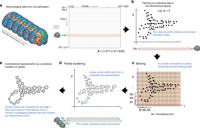
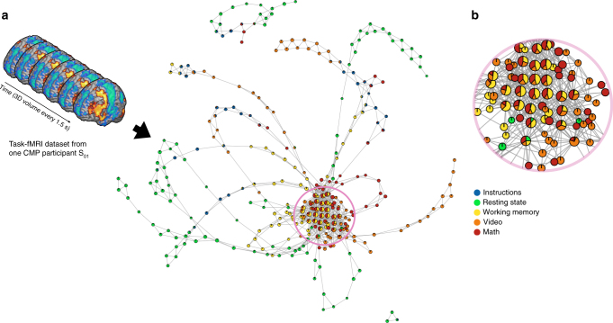
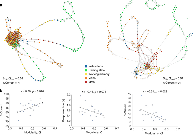
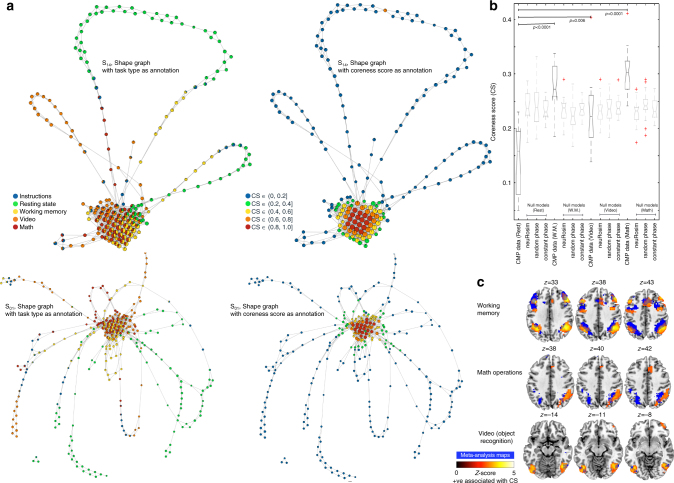
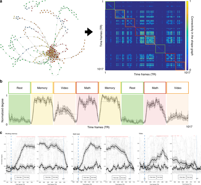
Little is known about how our brains dynamically adapt for efficient functioning. Most previous work has focused on analyzing changes in co-fluctuations between a set of brain regions over several temporal segments of the data. We argue that by collapsing data in space or time, we stand to lose useful information about the brain’s dynamical organization. Here we use Topological Data Analysis to reveal the overall organization of whole-brain activity maps at a single-participant level—as an interactive representation—without arbitrarily collapsing data in space or time. Using existing multitask fMRI datasets, with the known ground truth about the timing of transitions from one task-block to next, our approach tracks both within- and between-task transitions at a much faster time scale (~4–9 s) than before. The individual differences in the revealed dynamical organization predict task performance. In summary, our approach distills complex brain dynamics into interactive and behaviorally relevant representations.
Overview
The claims and statistics of this paper haven’t been checked yet.
Run the check — free, no account needed. It reads the open-access text and checks the sources it cites.
Integrity signals
Registry
Cites
Statistics
Figures
Verification
Claims the paper makes
The claims and statistics of this paper haven’t been checked yet.
Run the check — free, no account needed. It reads the open-access text and checks the sources it cites.
Claims other papers make about this one
Each is checked against this paper’s own text: does it say what the citing paper says it does?
In the citing paper
“Several recent studies have further shown how individual differences in task performance are related to patterns of dynamic brain organization54,55.”
From Cognitive and behavioural flexibility: Neural mechanisms and clinical considerations (2021) · cites this paper as [55]
Self-check
Percentages, sums and reported differences re-computed from the paper’s own numbers.
The self-check needs the paper’s full text.
Citations
Cites
(2008) · Journal of Machine Learning Research · Cited by 33,051
A Global Geometric Framework for Nonlinear Dimensionality Reduction
Tenenbaum, J. B., Silva, V. D., & Langford, J. C. (2000) · Science · doi:10.1126/science.290.5500.2319 · Cited by 13,585
Complex brain networks: graph theoretical analysis of structural and functional systems
Bullmore, E., & Sporns, O. (2009) · Nature Reviews Neuroscience · doi:10.1038/nrn2575 · Cited by 11,820
Self-citationFortunato, S. (2010) · Physics Reports · doi:10.1016/j.physrep.2009.11.002 · Cited by 11,293
Fast algorithm for detecting community structure in networks
Newman, M. E. J. (2004) · Physical Review E · doi:10.1103/physreve.69.066133 · Cited by 5,415
The minimal preprocessing pipelines for the Human Connectome Project
Glasser, M. F., Sotiropoulos, S. N., Wilson, J. A., Coalson, T. S., Fischl, B., Andersson, J. L., Xu, J., Jbabdi, S., Webster, M., Polimeni, J. R., et al. (2013) · NeuroImage · doi:10.1016/j.neuroimage.2013.04.127 · Cited by 5,253
Correspondence of the brain's functional architecture during activation and rest
Smith, S. M., Fox, P. T., Miller, K. L., Glahn, D. C., Fox, P. M., Mackay, C. E., Filippini, N., Watkins, K. E., Toro, R., Laird, A. R., et al. (2009) · Proceedings of the National Academy of Sciences · doi:10.1073/pnas.0905267106 · Cited by 5,150
A component based noise correction method (CompCor) for BOLD and perfusion based fMRI
Behzadi, Y., Restom, K., Liau, J., & Liu, T. T. (2007) · NeuroImage · doi:10.1016/j.neuroimage.2007.04.042 · Cited by 4,502
Consistent resting-state networks across healthy subjects
Damoiseaux, J. S., Rombouts, S. A. R. B., Barkhof, F., Scheltens, P., Stam, C. J., Smith, S. M., & Beckmann, C. F. (2006) · Proceedings of the National Academy of Sciences · doi:10.1073/pnas.0601417103 · Cited by 4,326
Functional Network Organization of the Human Brain
Power, J. D., Cohen, A. L., Nelson, S. M., Wig, G. S., Barnes, K. A., Church, J. A., Vogel, A. C., Laumann, T. O., Miezin, F. M., Schlaggar, B. L., et al. (2011) · Neuron · doi:10.1016/j.neuron.2011.09.006 · Cited by 4,124
Cited by
Sorted by citations
Items 101–200 of 251
Adaptive Covers for Mapper Graphs Using Information Criteria
Chalapathi, N., Zhou, Y., & Wang, B. (2021) · IEEE International Conference on Big Data (BigData) · doi:10.1109/bigdata52589.2021.9671324 · Cited by 8
Lin, B. (2022) · Algorithms · doi:10.3390/a15100371 · Cited by 10
The topological properties of the protein universe
Madsen, C. D., Barbensi, A., Zhang, S. Y., Ham, L., David, A., Pires, D. E. V., & Stumpf, M. P. H. (2025) · Nature Communications · doi:10.1038/s41467-025-61108-2 · Cited by 7
Kang, S. J., & Lim, Y. (2021) · Stat · doi:10.1002/sta4.405 · Cited by 7
V-Mapper: topological data analysis for high-dimensional data with velocity
Imoto, Y., & Hiraoka, Y. (2023) · Nonlinear Theory and Its Applications IEICE · doi:10.1587/nolta.14.92 · Cited by 9
The topology of data hides in quantum thermal states
Scali, S., Umeano, C., & Kyriienko, O. (2024) · APL Quantum · doi:10.1063/5.0209201 · Cited by 15
Siva, N. K., Singh, Y., Hathaway, Q. A., Sengupta, P. P., & Yanamala, N. V. K. (2024) · Scientific Reports · doi:10.1038/s41598-024-61201-4 · Cited by 7
𝓗1 persistent features of the resting-state connectome in healthy subjects
Martínez, D., Gonzalez, F. A., & Gómez, F. (2022) · Network Neuroscience · doi:10.1162/netn_a_00280 · Cited by 7
Kumar, S., Shovon, A. R., & Deshpande, G. (2023) · Human Brain Mapping · doi:10.1002/hbm.26403 · Cited by 10
Fingerprints of cancer by persistent homologyPreprint
Carpio, A., Bonilla, L. L., Mathews, J. C., & Tannenbaum, A. (2019) · bioRxiv (Cold Spring Harbor Laboratory) · doi:10.1101/777169 · Cited by 7
Topological data analysis for revealing dynamic brain reconfiguration in MEG data
Duman, A. N., & Tatar, A. E. (2023) · PeerJ · doi:10.7717/peerj.15721 · Cited by 6
Topological analysis of the latent geometry of a complex network
Jhun, B. (2022) · Chaos An Interdisciplinary Journal of Nonlinear Science · doi:10.1063/5.0073107 · Cited by 7
Functional neuroimaging in the era of Big Data and Open Science: A modern overview
Lazar, N. A. (2023) · Wiley Interdisciplinary Reviews Computational Statistics · doi:10.1002/wics.1609 · Cited by 6
Chung, M. K., Azizi, T., Hanson, J. L., Alexander, A. L., Pollak, S. D., & Davidson, R. J. (2023) · Network Neuroscience · doi:10.1162/netn_a_00355 · Cited by 11
NeuroDesign: Greater than the Sum of Its Parts
Auernhammer, J. M. K., Bruno, J. L., Booras, A., McIntyre, C., Haşegan, D., & Saggar, M. (2023) · Understanding innovation · doi:10.1007/978-3-031-36103-6_10 · Cited by 6
Self-citationde Alteriis, G., MacNicol, E., Hancock, F., Ciaramella, A., Cash, D., Expert, P., & Turkheimer, F. (2024) · Imaging Neuroscience · doi:10.1162/imag_a_00113 · Cited by 6
Kulkarni, A. P., Chung, M. K., Bendlin, B. B., & Prabhakaran, V. (2020) · doi:10.1109/isbiworkshops50223.2020.9153361 · Cited by 6
Topological insights into the neural basis of flexible behavior
Rouse, T. C., Ni, A. M., Huang, C., & Cohen, M. R. (2023) · Proceedings of the National Academy of Sciences · doi:10.1073/pnas.2219557120 · Cited by 8
Catanzaro, M. J., Rizzo, S., Kopchick, J. J., Chowdury, A., Rosenberg, D. R., Bubenik, P., & Diwadkar, V. A. (2023) · Neuroinformatics · doi:10.1007/s12021-023-09645-3 · Cited by 6
Simplicial complex entropy for time series analysis
Guzmán-Vargas, L., Zabaleta-Ortega, Á., & Guzmán-Sáenz, A. (2023) · Scientific Reports · doi:10.1038/s41598-023-49958-6 · Cited by 5
Wang, Y., Xian, J., Chen, Y., & Yan, Y. (2025) · Frontiers in Human Neuroscience · doi:10.3389/fnhum.2025.1607941 · Cited by 6
Can fMRI functional connectivity index dynamic neural communication and cognition?
Alonso, S., Llera, A., ter Horst, G., & Vidaurre, D. (2025) · Biological Psychology · doi:10.1016/j.biopsycho.2025.109074 · Cited by 6
Topological Data Analysis for Network Resilience Quantification
Pereira, L. M., Torres, L. C., & Amini, M. H. (2021) · Operations Research Forum · doi:10.1007/s43069-021-00070-3 · Cited by 5
Singh, Y., Jons, W. A., Sobek, J. D., Eaton, J. E., Erickson, B. J., Anderies, B. J., & Jagtap, J. M. M. (2022) · IEEE Annual Computing and Communication Workshop and Conference (CCWC) · doi:10.1109/ccwc54503.2022.9720887 · Cited by 5
Quantum topological data analysis via the estimation of the density of states
Scali, S., Umeano, C., & Kyriienko, O. (2024) · Physical Review A · doi:10.1103/physreva.110.042616 · Cited by 11
Zulkepli, N. F. S., Madukpe, V. N., Noorani, M. S. M., Bakar, M. A. A., Gobithaasan, R. U., & Jie, O. C. (2024) · Air Quality Atmosphere & Health · doi:10.1007/s11869-024-01596-1 · Cited by 4
Abdulrasul, H., Brice, H., & Jasińska, K. K. (2025) · Developmental Cognitive Neuroscience · doi:10.1016/j.dcn.2025.101532 · Cited by 9
The Possibility Space Concept in Neuroscience: Possibilities, Constraints, and Explanations
Ross, L. N., Jirsa, V., & McIntosh, A. R. (2025) · European Journal of Neuroscience · doi:10.1111/ejn.70038 · Cited by 5
Comparing Mapper Graphs of Artificial Neuron Activations
Zhou, Y., Jenne, H., Brown, D., Shapiro, M. R., Jefferson, B. A., Joslyn, C., Henselman‐Petrusek, G., Praggastis, B., Purvine, E., & Wang, B. (2023) · Topological Data Analysis and Visualization (TopoInVis) · doi:10.1109/topoinvis60193.2023.00011 · Cited by 4
Bandettini, P. A. (2021) · Springer eBooks · doi:10.1007/978-3-030-59797-9_2 · Cited by 6
Self-citationSubject-Specific Brain Activity Analysis in fMRI Data Using Merge Trees
Rasheed, F., Jonsson, D., Nilsson, E., Masood, T. B., & Hotz, I. (2022) · Topological Data Analysis and Visualization (TopoInVis) · doi:10.1109/topoinvis57755.2022.00018 · Cited by 4
Fan, L., Li, Y., Huang, Z., Zhang, W., Wu, X., Liu, T., & Wang, J. (2023) · Cerebral Cortex · doi:10.1093/cercor/bhad228 · Cited by 4
Uncovering Brain Chaos with Hypergraph-Based Framework
Ramanathan, S., & Ramasundaram, M. (2020) · International Journal of Intelligent Systems and Applications · doi:10.5815/ijisa.2020.04.04 · Cited by 4
Elyasi, N., & Moghadam, M. H. (2019) · arXiv (Cornell University) · doi:10.48550/arxiv.1906.01726 · Cited by 4
Fujisawa, K., Kumano, M., & Kimura, M. (2023) · Applied Network Science · doi:10.1007/s41109-023-00577-0 · Cited by 3
Valerio, J., Filho, J. E. D. V., Stosic, B. D., de Oliveira, W. R., da Silva, F. M. S., Antonino, A. C. D., & Duarte‐Neto, P. J. (2024) · Micron · doi:10.1016/j.micron.2024.103731 · Cited by 3
Does topological data analysis work for EEG-based brain–computer interfaces?
Xu, X., Drougard, N., & Roy, R. N. (2025) · Journal of Neural Engineering · doi:10.1088/1741-2552/add8bd · Cited by 3
A Primer on Persistent Homology of Finite Metric Spaces
Mémoli, F., & Singhal, K. (2019) · Bulletin of Mathematical Biology · doi:10.1007/s11538-019-00614-z · Cited by 6
A covariate-constraint method to map brain feature space into lower dimensional manifolds
Renard, F., Heinrich, C., Bouthillon, M., Schenck, M., Schneider, F., Kremer, S., & Achard, S. (2020) · Network Neuroscience · doi:10.1162/netn_a_00176 · Cited by 5
Toda, A., Hiwa, S., Tanioka, K., & Hiroyasu, T. (2022) · IEEE Congress on Evolutionary Computation (CEC) · doi:10.1109/cec55065.2022.9870341 · Cited by 4
Visual number sense for real-world scenes shared by deep neural networks and humans
Wu, W., Ge, Y., Zuo, Z., Chen, L., Xu, Q., & Liu, Z. (2023) · Heliyon · doi:10.1016/j.heliyon.2023.e18517 · Cited by 5
Tree representations of brain structural connectivity via persistent homology
Li, D., Nguyen, P. H., Zhang, Z., & Dunson, D. B. (2023) · Frontiers in Neuroscience · doi:10.3389/fnins.2023.1200373 · Cited by 3
Kim, D., Kim, S., Kim, Y. D., & Lyu, S. (2025) · KSCE Journal of Civil Engineering · doi:10.1016/j.kscej.2025.100177 · Cited by 3
The topology of representational geometry
Brown, S. R., & Farivar, R. (2025) · Frontiers in Neuroscience · doi:10.3389/fnins.2025.1597899 · Cited by 3
Song, X., Bhinge, S., Quiton, R. L., & Adalı, T. (2019) · Journal of Neuroscience Methods · doi:10.1016/j.jneumeth.2019.108356 · Cited by 3
Topological Data Analysis for Classification of DeepSat-4 Dataset
Moghadam, M. H., & Pedram, M. M. (2020) · International Symposium on Telecommunications · doi:10.1109/ist50524.2020.9345829 · Cited by 3
Gao, Q. C., Xiang, Y., Zhang, J., Luo, N., Liang, M., Gong, L., Yu, J., Cui, Q., Sepulcre, J., & Chen, H. (2021) · NeuroImage · doi:10.1016/j.neuroimage.2021.118497 · Cited by 3
Persistent homology of collider observations: When (w)hole matters
Beuria, J. (2023) · Physics Letters B · doi:10.1016/j.physletb.2023.138188 · Cited by 3
de Alteriis, G., MacNicol, E., Hancock, F., Ciaramella, A., Cash, D., Expert, P., & Turkheimer, F. (2023) · bioRxiv (Cold Spring Harbor Laboratory) · doi:10.1101/2023.02.27.529688 · Cited by 3
Machine Learning Interpretability Methods to Characterize Brain Network Dynamics in EpilepsyPreprint
Upadhyaya, D. P., Prantzalos, K., Thyagaraj, S., Shafiabadi, N., Fernandez-BacaVaca, G., Sivagnanam, S., Majumdar, A., & Sahoo, S. S. (2023) · medRxiv · doi:10.1101/2023.06.25.23291874 · Cited by 3
Topological optimal transport for geometric cycle matching
Zhang, S. Y., Stumpf, M. P. H., Needham, T., & Barbensi, A. (2025) · Journal of Applied and Computational Topology · doi:10.1007/s41468-025-00207-x · Cited by 2
How to Probe Dynamics of Brain Function: A Narrative Review
Pushkarskaya, H., Krishnaswamy, S., & Pittenger, C. (2025) · Biological Psychiatry · doi:10.1016/j.biopsych.2025.11.023 · Cited by 2
A topological data analysis method for revealing dynamic changes in psychotherapy microprocesses
Luo, X., & Zhang, M. (2026) · Frontiers in Psychology · doi:10.3389/fpsyg.2025.1711782 · Cited by 2
A topological approach for semi-supervised learning
Inés, A., Domínguez, C., Heras, J. A. M., Mata, G., & Rubio, J. (2024) · Journal of Computational Science · doi:10.1016/j.jocs.2024.102403 · Cited by 2
A novel method for subgroup discovery in precision medicine based on topological data analysis
Loughrey, C. F., Maguire, S., Dłotko, P., Bai, L., Orr, N., & Jurek, A. (2025) · BMC Medical Informatics and Decision Making · doi:10.1186/s12911-025-02852-9 · Cited by 2
Chen, Y., Qin, D., & Kuruoğlu, E. E. (2025) · Lecture notes in computer science · doi:10.1007/978-981-96-3294-7_16 · Cited by 2
Studying Task-Modulated Functional Connectivity Using Functional Magnetic Resonance Imaging
Masharipov, R. S., Didour, M., Cherednichenko, D. V., & Kireev, M. V. (2026) · Neuroscience and Behavioral Physiology · doi:10.1007/s11055-026-01954-9 · Cited by 2
Time-resolved analysis of dynamic graphs: an extended Slepian design
Liégeois, R., Merad, I., & Ville, D. V. D. (2019) · Wavelets and Sparsity · doi:10.1117/12.2530550 · Cited by 2
Measuring intrinsic significance of community structure
Xie, J., Du, M., Di, Z., Zhu, H., Fan, Y., & Hu, Y. (2019) · International Journal of Modern Physics C · doi:10.1142/s0129183119500682 · Cited by 2
Isojima, S., Tanioka, K., Hiroyasu, T., & Hiwa, S. (2023) · International Journal of Intelligent Transportation Systems Research · doi:10.1007/s13177-023-00371-3 · Cited by 2
Intrinsic geometry of collider observations and forman Ricci curvature
Beuria, J. (2023) · Physical Review D · doi:10.1103/physrevd.110.035023 · Cited by 5
Thompson, W. H., Wright, J., Shine, J. M., & Poldrack, R. A. (2019) · bioRxiv (Cold Spring Harbor Laboratory) · doi:10.1101/617027 · Cited by 2
Brain mitochondrial diversity and network organization predict anxiety-like behavior in micePreprint
Rosenberg, A. M., Saggar, M., Monzel, A. S., Devine, J., Rogu, P. J., Limoges, A., Junker, A., Sandi, C., Mosharov, E. V., Dumitriu, D., et al. (2021) · bioRxiv (Cold Spring Harbor Laboratory) · doi:10.1101/2021.06.02.446767 · Cited by 2
Self-citationThe decomposition of the higher-order homology embedding constructed from the $k$-LaplacianPreprint
Chen, Y., & Meilă, M. (2021) · arXiv (Cornell University) · doi:10.48550/arxiv.2107.10970 · Cited by 2
Topology of the mesoscale connectome of the mouse brain
Grange, P. (2020) · Computational and Mathematical Biophysics · doi:10.1515/cmb-2020-0106 · Cited by 2
Liu, C., Ma, X., Zhang, H., Xie, S., & Yu, D. (2024) · IEEE Access · doi:10.1109/access.2024.3446281 · Cited by 1
Zuo, W., Fang, S., Xu, T., Li, Y., Zhao, J., Xie, X., Wang, T., Hou, W., & Wang, M. (2025) · CNS Neuroscience & Therapeutics · doi:10.1111/cns.70271 · Cited by 1
Methods for Brain Connectivity Analysis with Applications to Rat Local Field Potential Recordings
El-Yaagoubi, A. B., Aslan, S., Gomawi, F., Redondo, P. V., Roy, S., Sultan, M. S., Talento, M. S., Tarrazona, F. T., Wu, H., Cooper, K. W., et al. (2025) · Entropy · doi:10.3390/e27040328 · Cited by 1
Zhang, M., Li, H., Bai, S., Nan, X., Ma, N., Liu, R., & Wen, Q. (2025) · Physics of Fluids · doi:10.1063/5.0280985 · Cited by 1
Shovon, A. R., Kumar, S., & Deshpande, G. (2025) · IEEE Access · doi:10.1109/access.2025.3616256 · Cited by 1
MapperEEG: A topological approach to brain state clustering in EEG recordings
Story, B., Zhou, Z., Srinivasan, R., Kerick, S. E., Boothe, D. L., & Franaszczuk, P. J. (2026) · Journal of Neuroscience Methods · doi:10.1016/j.jneumeth.2026.110744 · Cited by 1
Kilic, B. Ü., Jubeir, J., Balchandani, P., Murrough, J. W., Morris, L. S., & Jacob, Y. (2026) · Nature Communications · doi:10.1038/s41467-026-71961-4 · Cited by 1
Charting higher-order models of brain function beyond pairwise interactions
Santoro, A., Neri, M., Poetto, S., Orsenigo, D., Diano, M., Gatica, M., & Petri, G. (2026) · Nature Communications · doi:10.1038/s41467-026-75959-w · Cited by 1
Exploration of Mapper-A Method for Topological Data Analysis
Sun, C. (2020) · International Conference on Information Science, Parallel and Distributed Systems (ISPDS) · doi:10.1109/ispds51347.2020.00036 · Cited by 1
Examining the Neurocognitive Basis of Applied Creativity in Entrepreneurs and Managers
Auernhammer, J. M. K., Sonalkar, N., Xie, H., Monlux, K. D., Bruno, J. L., & Saggar, M. (2021) · Understanding innovation · doi:10.1007/978-3-030-76324-4_18 · Cited by 1
Self-citationGraph Theory for Brain Signal Processing
Laskaris, N., Adamos, D. A., & Bezerianos, A. (2021) · Handbook of Neuroengineering · doi:10.1007/978-981-15-2848-4_66-2 · Cited by 1
The Euler characteristic as a topological marker for outbreaks in vector-borne disease
de Souza, D. B., dos Santos, E. F., & Santos, F. A. N. (2022) · Journal of Statistical Mechanics Theory and Experiment · doi:10.1088/1742-5468/aca0e5 · Cited by 1
Offroy, M., Duponchel, L., Razafitianamaharavo, A., Pagnout, C., & Duval, J. F. L. (2024) · Talanta · doi:10.1016/j.talanta.2024.127482 · Cited by 1
Piecewise Computation of Persistent Homology
Singh, R. P., Malott, N. O., & Wilsey, P. A. (2024) · IEEE International Conference on Big Data (BigData) · doi:10.1109/bigdata62323.2024.10825374 · Cited by 1
Implementing evolutionary optimization to model neural functional connectivity
Maile, K., Saggar, M., & Miikkulainen, R. P. (2019) · Genetic and Evolutionary Computation Conference Companion (GECCO Companion) · doi:10.1145/3319619.3326826 · Cited by 1
Self-citationMining the Role of Design Reflection and Associated Brain Dynamics in Creativity
Sonalkar, N., Jahanikia, S., Xie, H., Geniesse, C., Ayub, R., Beaty, R. E., & Saggar, M. (2019) · Understanding innovation · doi:10.1007/978-3-030-28960-7_10 · Cited by 1
Self-citationSpatial Perception for Structured and Unstructured Data In topological Data Analysis
Kitanishi, Y., Ishioka, F., Iizuka, M., & Kurihara, K. (2021) · Studies in classification, data analysis, and knowledge organization · doi:10.1007/978-3-030-60104-1_12 · Cited by 1
A Python Hands-on Tutorial on Network and Topological Neuroscience
Centeno, E. G. Z., Moreni, G., Vriend, C., Douw, L., & Santos, F. A. N. (2021) · Lecture notes in computer science · doi:10.1007/978-3-030-80209-7_71 · Cited by 1
Stitch Fix for Mapper and Topological Gains
Zhou, Y., Saul, N., Safarli, I., Krishnamoorthy, B., & Wang, B. (2022) · Association for Women in Mathematics series · doi:10.1007/978-3-030-95519-9_12 · Cited by 1
Higher-Order Description of Brain Function
Expert, P., & Petri, G. (2022) · Understanding complex systems · doi:10.1007/978-3-030-91374-8_17 · Cited by 1
Graph Theory for Brain Signal Processing
Laskaris, N., Adamos, D. A., & Bezerianos, A. (2023) · Handbook of Neuroengineering · doi:10.1007/978-981-16-5540-1_66 · Cited by 2
Fujisawa, K., Kumano, M., & Kimura, M. (2023) · Studies in computational intelligence · doi:10.1007/978-3-031-21131-7_48 · Cited by 1
Feasibility of Topological Data Analysis for event-related fMRIPreprint
Ellis, C. T., Lesnick, M., Henselman‐Petrusek, G., Keller, B., & Cohen, J. D. (2018) · bioRxiv (Cold Spring Harbor Laboratory) · doi:10.1101/457747 · Cited by 1
Resting-state fMRI Signals of Intelligent People Wander in a Larger SpacePreprint
Dizaji, A. S., Khodaei, M., & Hamid Soltanian-zadeh, A. (2019) · bioRxiv (Cold Spring Harbor Laboratory) · doi:10.1101/529362 · Cited by 1
A Tutorial on Graph Theory for Brain Signal AnalysisPreprint
Laskaris, N., Adamos, D. A., & Bezerianos, A. (2020) · arXiv (Cornell University) · doi:10.48550/arxiv.2007.05800 · Cited by 1
Persistent Homology of Weighted Visibility Graph from Fractional Gaussian Noise.Preprint
Masoomy, H., Askari, B., Najafi, M. N., & Movahed, M. S. (2021) · arXiv (Cornell University) · Cited by 1
Can fMRI functional connectivity index dynamic neural communication?Preprint
Alonso, S., Llera, A., ter Horst, G., & Vidaurre, D. (2021) · bioRxiv (Cold Spring Harbor Laboratory) · doi:10.1101/2021.07.27.453965 · Cited by 1
Jeong, G., & Paolini, M. (2022) · bioRxiv (Cold Spring Harbor Laboratory) · doi:10.1101/2022.08.30.505423 · Cited by 1
Manifold Learning for fMRI time-varying FCPreprint
González-Castillo, J., Fernandez, I. S., Lam, K. C., Handwerker, D. A., Pereira, F., & Bandettini, P. A. (2023) · bioRxiv (Cold Spring Harbor Laboratory) · doi:10.1101/2023.01.14.523992 · Cited by 1
Self-citationInvestigating the Nonlinear Dynamics of Human Balance Using Topological Data Analysis
Siegrist, K. W., Chagdes, J. R., & Kramer, R. M. (2019) · doi:10.1115/detc2019-98014
Persistent Homology for Dimensionality Reduction
Williamson, L. (2021) · Studies in computational intelligence · doi:10.1007/978-3-030-41188-6_9
Zhang, Y., Farrugia, N., Dagher, A., & Bellec, P. (2021) · bioRxiv (Cold Spring Harbor Laboratory) · doi:10.1101/2021.07.26.453914
Multivariate characterization of brain dynamics for disorders of consciousness
Castaño, R., & Eliécer, J. (2021)
Topological insights into the neural basis of flexible behaviorPreprint
Rouse, T. C., Ni, A. M., Huang, C., & Cohen, M. R. (2021) · bioRxiv (Cold Spring Harbor Laboratory) · doi:10.1101/2021.09.24.461717
LEIFER, L. J., & Meinel, C. (2019) · Understanding innovation · doi:10.1007/978-3-030-28960-7_1
Metadata
- Authors
- Saggar, M., Sporns, O., Gonzalez-Castillo, J., Bandettini, P. A., Carlsson, G., Glover, G., & Reiss, A. L.
- Affiliations
- Stanford Medicine (US)
- Indiana University Bloomington (US)
- National Institutes of Health (US)
- Ayasdi (United States) (US)
- Stanford University (US)
- Corresponding author
- Saggar, Manish
- Venue
- Nature Communications
- Published
- 2018-04-11
- Volume
- 9
- Issue
- 1
- Pages
- 1399-1399
- ISSN
- 2041-1723 (ISSN-L)
- PMC
- PMC5895632
- OpenAlex
- W2797507693
- Cited by
- 253
- References
- 69
- Citations by year
- 2026: 29 · 2025: 32 · 2024: 19 · 2023: 40 · 2022: 24 · 2021: 40 · 2020: 27 · 2019: 32 · 2018: 10
- FWCI
- 16.23
- Type
- journal article
- Language
- en
- Open access
- gold
- doi.org
- Locations
- Nature Communications (publishedVersion, cc-by)
- Europe PMC (PubMed Central) (publishedVersion, other-oa)
- PubMed Central (publishedVersion, cc-by)
- PubMed (publishedVersion)
- RePEc: Research Papers in Economics (submittedVersion)
- DOAJ (DOAJ: Directory of Open Access Journals) (submittedVersion)
- DOAJ (DOAJ: Directory of Open Access Journals) (submittedVersion, cc-by-sa)
- IUScholarWorks Open (Indiana University) (submittedVersion)
- Funders
- National Alliance for Research on Schizophrenia and Depression
- National Institutes of Health (93-M-0170, NCT00001360, 5u54mh091657-05, 1U54‐MH‐091657)
- McDonnell Center for Systems Neuroscience (ZIAMH002783, 1U54MH091657)
- National Institute of Mental Health (K99MH104605, 1U54 MH091657, U54-MH091657, 93- M-0170, NCT00001360, R00MH104605, ZIAMH002783)
- Topics
- Life Sciences › Neuroscience › Cognitive Neuroscience › Functional Brain Connectivity Studies
- Physical Sciences › Computer Science › Computational Theory and Mathematics › Topological and Geometric Data Analysis
- Life Sciences › Neuroscience › Cognitive Neuroscience › Neural dynamics and brain function
- Keywords
- brain dynamics, topological data analysis, task transitions, interactive visualization, individual differences, task performance prediction
- MeSH terms
- Adult, Brain, Female, Humans, Magnetic Resonance Imaging, Male, Memory, Short-Term, Nerve Net, Rest, Task Performance and Analysis, Connectome, Datasets as Topic
About these checks
Registry, retraction, Cites and statistics results are computed, not judged, with one exception: a printed reference that no index lists is read once by a model before it counts as a citation error. Claims are extracted by a model and kept only when their quote appears verbatim in the text; each cited source is then checked, with a model’s help, for whether it says what the claim relies on. Those verdicts can be wrong — read the claim’s quote and the cited source before relying on one.
Statistics and arithmetic are recomputed, not judged.
Confidence bands are shown only for fields calibrated on our annotated test set. None is calibrated yet, so no band is shown.
What counts as a claim ›How we measure confidence ›How we check this ›
Are you an author, or do you see a problem with this page? Request a review
