Student or educator? Sign up with your school email and get 6 months of Pro free.
CoChat

The DOI matches its Crossref record; 78 of the 78 references it cites were found in a registry or an index.

Clone-structured graph representations enable flexible learning and vicarious evaluation of cognitive maps

Open access

Abstract

Cognitive maps are mental representations of spatial and conceptual relationships in an environment, and are critical for flexible behavior. To form these abstract maps, the hippocampus has to learn to separate or merge aliased observations appropriately in different contexts in a manner that enables generalization and efficient planning. Here we propose a specific higher-order graph structure, clone-structured cognitive graph (CSCG), which forms clones of an observation for different contexts as a representation that addresses these problems. CSCGs can be learned efficiently using a probabilistic sequence model that is inherently robust to uncertainty. We show that CSCGs can explain a variety of cognitive map phenomena such as discovering spatial relations from aliased sensations, transitive inference between disjoint episodes, and formation of transferable schemas. Learning different clones for different contexts explains the emergence of splitter cells observed in maze navigation and event-specific responses in lap-running experiments. Moreover, learning and inference dynamics of CSCGs offer a coherent explanation for disparate place cell remapping phenomena. By lifting aliased observations into a hidden space, CSCGs reveal latent modularity useful for hierarchical abstraction and planning. Altogether, CSCG provides a simple unifying framework for understanding hippocampal function, and could be a pathway for forming relational abstractions in artificial intelligence.

Overview

The claims and statistics of this paper haven’t been checked yet.

Free: it reads the open-access text and checks the first 5 claims that cite a source we can check. Create a free account to check every claim.

A few free checks a day · papers already verified open instantly · results are public

Integrity signals

Registry

Crossref · 10.1038/s41467-021-22559-5

Cites

78 of 78 references verified0 citation errors · 0 not checkable

Statistics

Figures

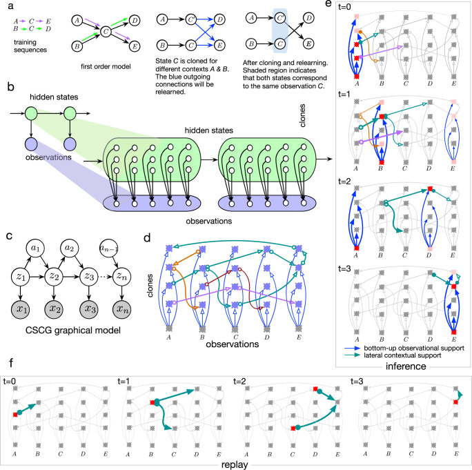
Fig. 1 Clone-structured cognitive graph. a Sketch explaining dynamic Markov coding. A first-order Markov chain shown as a graph between nodes representing its states, modeling observation sequences A → C → E (purple arrows) and B → C → D (green arrows) will also assign high probability to the sequence A → C → D because higher-order information is lost at state C. (Middle) Higher-order information can be recovered by cloning the state C for different contexts, and then relearning their outgoing connections (blue) to result in the graph on the right. b Cloning structure of dynamic Markov coding can be represented in an HMM with a structured emission matrix, the cloned HMM. c Probabilistic graphical model for CSCG which extends cloned HMMs in b by including actions. d Neural implementation of cloned HMM. Arrows are axons, and the lateral connections implement the cloned HMM transition matrix. Different sequences are in different colors, e.g., A → C → E in purple. Neurons in a column are clones of each other that receive the bottom-up input (blue arrows) from the same observation. e Inference dynamics in the cloned HMM neural circuit. Neural activations strengths are represented in shades of red. Activations that propagate forward are the ones that have contextual (lateral) and observational (bottom-up) support. f Replay within the circuit for the sequence A → B → (C, D) → E → E.
Fig. 1 Clone-structured cognitive graph. a Sketch explaining dynamic Markov coding. A first-order Markov chain shown as a graph between nodes representing its states, modeling observation sequences A → C → E (purple arrows) and B → C → D (green arrows) will also assign high probability to the sequence A → C → D because higher-order information is lost at state C. (Middle) Higher-order information can be recovered by cloning the state C for different contexts, and then relearning their outgoing connections (blue) to result in the graph on the right. b Cloning structure of dynamic Markov coding can be represented in an HMM with a structured emission matrix, the cloned HMM. c Probabilistic graphical model for CSCG which extends cloned HMMs in b by including actions. d Neural implementation of cloned HMM. Arrows are axons, and the lateral connections implement the cloned HMM transition matrix. Different sequences are in different colors, e.g., A → C → E in purple. Neurons in a column are clones of each other that receive the bottom-up input (blue arrows) from the same observation. e Inference dynamics in the cloned HMM neural circuit. Neural activations strengths are represented in shades of red. Activations that propagate forward are the ones that have contextual (lateral) and observational (bottom-up) support. f Replay within the circuit for the sequence A → B → (C, D) → E → E.CC BY · PubMed Central
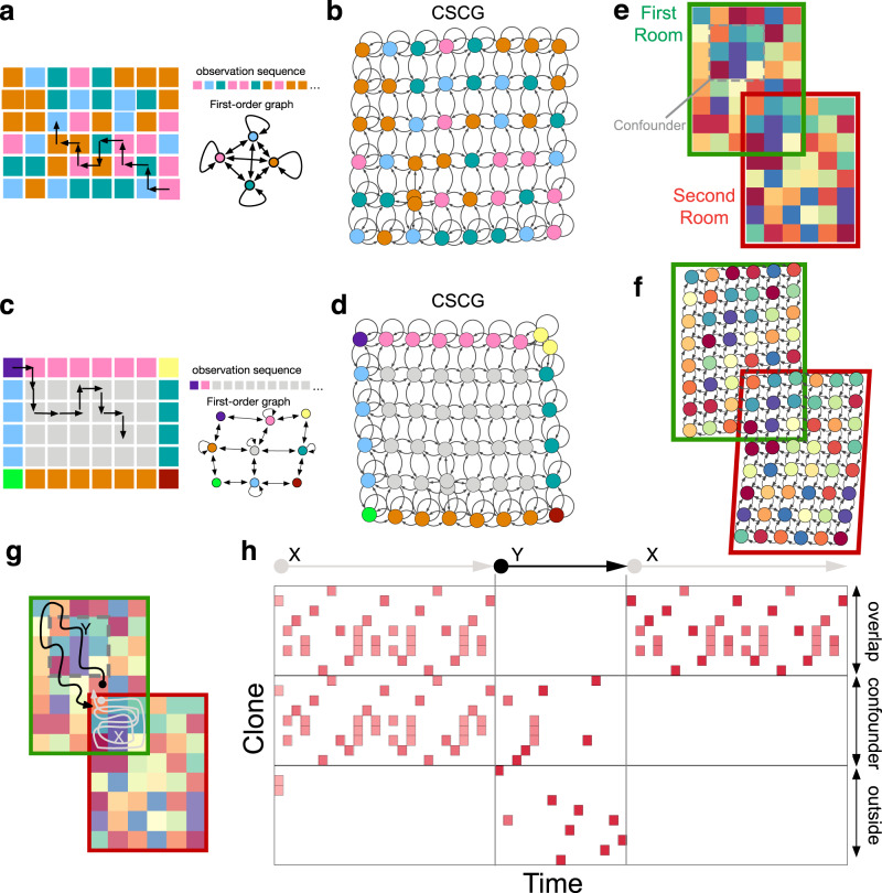
Fig. 2 Spatial representations emerge from aliased sequential random walk observations without Euclidean assumptions. a A random walk in a room with only four unique observations (colors) will produce a severely aliased sequence as reflected in the first-order Markov chain. b In contrast, transition graph learned by CSCG on random walks in a recovers the spatial layout. Nodes in this graph are the clones, and the observation they connect to are indicated by the color of the node. c Room with a uniform interior produces aliased sequences highly correlated in time. d Transition graph learned by CSCG on random walks in c, represented similar to b. The redundant yellow nodes (and some brown nodes in b) are due to slight imperfections in learning, but do not affect the representation or behavior. e An agent experiences two different, but overlapping rooms in disjoint sequential episodes. The overlap region also repeats in the first room, acting as a confounder. f As reflected in the transition graph, CSCG performs transitive inference to stitch together the disjoint experience into a coherent global map, and correctly positions the confounder. g, h Activation of clones over time as the agent takes the trajectories X (gray), Y (black), and X again in the maze in g. Each red square is a clone activation in one time step. During the first traversal of X, the clones corresponding to the overlap and the confounding patch are active because the agent started within the overlap and stayed within. Stepping outside the overlap immediately resolves ambiguity, which is reflected in the clone activity during the traversal Y which includes confounder region and areas outside overlap and confounder, and also during the second traversal of X. See also Supplementary Video 1.
Fig. 2 Spatial representations emerge from aliased sequential random walk observations without Euclidean assumptions. a A random walk in a room with only four unique observations (colors) will produce a severely aliased sequence as reflected in the first-order Markov chain. b In contrast, transition graph learned by CSCG on random walks in a recovers the spatial layout. Nodes in this graph are the clones, and the observation they connect to are indicated by the color of the node. c Room with a uniform interior produces aliased sequences highly correlated in time. d Transition graph learned by CSCG on random walks in c, represented similar to b. The redundant yellow nodes (and some brown nodes in b) are due to slight imperfections in learning, but do not affect the representation or behavior. e An agent experiences two different, but overlapping rooms in disjoint sequential episodes. The overlap region also repeats in the first room, acting as a confounder. f As reflected in the transition graph, CSCG performs transitive inference to stitch together the disjoint experience into a coherent global map, and correctly positions the confounder. g, h Activation of clones over time as the agent takes the trajectories X (gray), Y (black), and X again in the maze in g. Each red square is a clone activation in one time step. During the first traversal of X, the clones corresponding to the overlap and the confounding patch are active because the agent started within the overlap and stayed within. Stepping outside the overlap immediately resolves ambiguity, which is reflected in the clone activity during the traversal Y which includes confounder region and areas outside overlap and confounder, and also during the second traversal of X. See also Supplementary Video 1.CC BY · PubMed Central
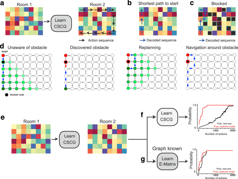
Fig. 3 Learned transition graphs form a reusable schema. A CSCG trained on one room (a) and partial observations in a second, previously unseen room with identical hidden layout, utilizes the learned structure of the room to rapidly find both the shortest path to the origin (b) and navigate around obstacles (c). d Visualization of message propagation during planning and replanning. Messages propagate outward from the starting clone, and clones that receive the message are indicated in green color. Lighter shades indicate messages that are later in time. The first plan is unaware of the obstacle, and the agent discovers the obstacle only when the action sequence is executed and a planned action fails (red arrow). This initiates a replanning from the new location, and the new plan routes around the obstacle. e–g The transition matrix (graph) learned in one room can be used as a reusable structure to quickly learn a new room with the same layout but different observations. Learning is faster when CSCG transition graph is used as a schema to learn the new room (g) compared to learning from scratch (f).
Fig. 3 Learned transition graphs form a reusable schema. A CSCG trained on one room (a) and partial observations in a second, previously unseen room with identical hidden layout, utilizes the learned structure of the room to rapidly find both the shortest path to the origin (b) and navigate around obstacles (c). d Visualization of message propagation during planning and replanning. Messages propagate outward from the starting clone, and clones that receive the message are indicated in green color. Lighter shades indicate messages that are later in time. The first plan is unaware of the obstacle, and the agent discovers the obstacle only when the action sequence is executed and a planned action fails (red arrow). This initiates a replanning from the new location, and the new plan routes around the obstacle. e–g The transition matrix (graph) learned in one room can be used as a reusable structure to quickly learn a new room with the same layout but different observations. Learning is faster when CSCG transition graph is used as a schema to learn the new room (g) compared to learning from scratch (f).CC BY · PubMed Central
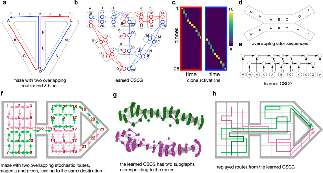
Fig. 4 Learning temporal order and paths. In all experiments, CSCG learned the optimal model for prediction, and the learned circuits matched neurobiological observations. a Modified T maze from16 with an overlapping segment between the blue and red paths. A, B, ⋯ , N are the observations at different locations in the maze. b CSCG learns route-differentiated clones for the overlapping segment. (The redundant clones on the non-overlapping segments are identical, and due to the learning algorithm not always using the minimal number of clones). c Activity of the clones for the right trial, and the left trial. Similar to the observations in16, the activity of clones in this overlapping segment will indicate whether the agent is going to turn left or right. Distinct neurons are active in the overlapping segment for left-turn trials vs right-turn trials although the observations in the overlapping segment are identical for both trials. Note that clones are not limited to one time step. CSCG learning is able to propagate clones backward into multiple time steps to unravel long overlapping paths. d Overlapping odor sequences from74 e Full circuit learned by the CSCG shows that it has learned distinct paths in the overlap, as in74. f A complex maze in which the agent takes two stochastic paths indicated in magenta and green. Observations in the maze are marked by numbers and, as before, the same observation can be sensed in many parts of the maze. The green and magenta paths overlap in up to seven locations in the middle segment (observations 4-5-11-12-13-5-17). The stochasticity of the paths and the long overlaps make this a challenging learning problem. In contrast to mazes in a and d, the two paths in this maze lead to the same destination as in20 g. Transition graph learned by the CSCG shows that two different chains are learned for the two routes in f, similar to the observation that place cells encode routes, not destinations20. h Paths replayed from the CSCG after it was trained on sequences from f. As they pass through the overlapping segment, the green and magenta routes maintain the higher-order history of where they originated, showing that the learned graph compactly represents the stochasticity and directionality of each route while separating the two routes by appropriately merging and splitting the clones.
Fig. 4 Learning temporal order and paths. In all experiments, CSCG learned the optimal model for prediction, and the learned circuits matched neurobiological observations. a Modified T maze from16 with an overlapping segment between the blue and red paths. A, B, ⋯ , N are the observations at different locations in the maze. b CSCG learns route-differentiated clones for the overlapping segment. (The redundant clones on the non-overlapping segments are identical, and due to the learning algorithm not always using the minimal number of clones). c Activity of the clones for the right trial, and the left trial. Similar to the observations in16, the activity of clones in this overlapping segment will indicate whether the agent is going to turn left or right. Distinct neurons are active in the overlapping segment for left-turn trials vs right-turn trials although the observations in the overlapping segment are identical for both trials. Note that clones are not limited to one time step. CSCG learning is able to propagate clones backward into multiple time steps to unravel long overlapping paths. d Overlapping odor sequences from74 e Full circuit learned by the CSCG shows that it has learned distinct paths in the overlap, as in74. f A complex maze in which the agent takes two stochastic paths indicated in magenta and green. Observations in the maze are marked by numbers and, as before, the same observation can be sensed in many parts of the maze. The green and magenta paths overlap in up to seven locations in the middle segment (observations 4-5-11-12-13-5-17). The stochasticity of the paths and the long overlaps make this a challenging learning problem. In contrast to mazes in a and d, the two paths in this maze lead to the same destination as in20 g. Transition graph learned by the CSCG shows that two different chains are learned for the two routes in f, similar to the observation that place cells encode routes, not destinations20. h Paths replayed from the CSCG after it was trained on sequences from f. As they pass through the overlapping segment, the green and magenta routes maintain the higher-order history of where they originated, showing that the learned graph compactly represents the stochasticity and directionality of each route while separating the two routes by appropriately merging and splitting the clones.CC BY · PubMed Central
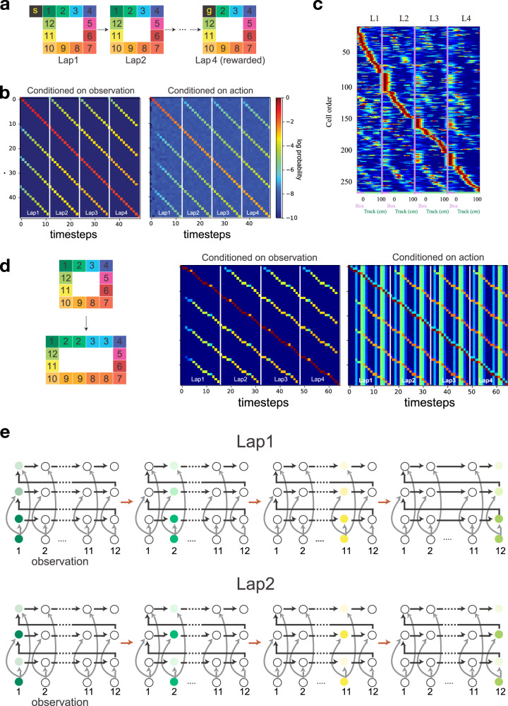
Fig. 5 Lap-neurons and event-specific representations. a A CSCG was trained on observations from four laps around a square maze similar to21. The training sequence consisted of one start state, followed by four repetitions of the sequence 1 → 2 → 3, .., 12, and then a goal/reward state at the end. It learned to predict the laps perfectly, including the reward at the end of the fourth lap, and planning to get the reward returned the correct sequence of actions. b Clone activations (see color map) for the four different laps. Rows correspond to clones. The activations show that there are different clones that are maximally active for different laps, but the other clones are partially active at their corresponding locations, similar to the neurophysiological observations in21 regarding event-specific-representations. c Place cell traces from21, included with permission. d The event-specific representations persist even when the maze is elongated by repeating the observations along the corridor. The CSCG is not trained on the elongated maze. e Visualization of the circuit learned by the CSCG including the transition graph, connections from the observations, and activation sequences for laps 1 and 2. The CSCG learned one clone per lap for each position. Smoothing in the CSCG explains why other clones of other laps are partially active. Each row shows how the clone activations transition from observation 1 (left) to observation 12 (right) for the corresponding lap. The active observations are colored in correspondence with a, and clone activations are graded in intensity with darker shades being stronger. Overall the visualizations show the circuit dynamics that give rise to the activity traces in b.
Fig. 5 Lap-neurons and event-specific representations. a A CSCG was trained on observations from four laps around a square maze similar to21. The training sequence consisted of one start state, followed by four repetitions of the sequence 1 → 2 → 3, .., 12, and then a goal/reward state at the end. It learned to predict the laps perfectly, including the reward at the end of the fourth lap, and planning to get the reward returned the correct sequence of actions. b Clone activations (see color map) for the four different laps. Rows correspond to clones. The activations show that there are different clones that are maximally active for different laps, but the other clones are partially active at their corresponding locations, similar to the neurophysiological observations in21 regarding event-specific-representations. c Place cell traces from21, included with permission. d The event-specific representations persist even when the maze is elongated by repeating the observations along the corridor. The CSCG is not trained on the elongated maze. e Visualization of the circuit learned by the CSCG including the transition graph, connections from the observations, and activation sequences for laps 1 and 2. The CSCG learned one clone per lap for each position. Smoothing in the CSCG explains why other clones of other laps are partially active. Each row shows how the clone activations transition from observation 1 (left) to observation 12 (right) for the corresponding lap. The active observations are colored in correspondence with a, and clone activations are graded in intensity with darker shades being stronger. Overall the visualizations show the circuit dynamics that give rise to the activity traces in b.CC BY · PubMed Central
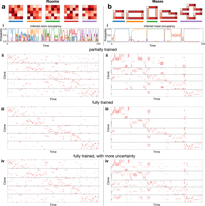
Fig. 6 Remapping. Sets consisting of five different rooms (a) and mazes (b) are used to study activity remapping. In set a, the five rooms share 25 different observations, arranged randomly, and in set b, the five mazes share six observations arranged in geometrical shapes. Different shades of red represent different observations. Row (i): inferred probability (Y-axis) of being in a room/maze as a function of time (X-axis). Rows (ii)–(iv) Clone activity traces for a random walk of 50 steps each in rooms (mazes) 1–5 under different conditions (partially trained, fully trained, and more uncertainty). All traces are based on the same random walk and use the same clone ordering. Activity traces corresponds to global remapping in a partially trained CSCG, and partial remapping in a partially trained CSCG. Adding more uncertainty to a fully trained CSCG produces activity traces that correspond to rate remapping.
Fig. 6 Remapping. Sets consisting of five different rooms (a) and mazes (b) are used to study activity remapping. In set a, the five rooms share 25 different observations, arranged randomly, and in set b, the five mazes share six observations arranged in geometrical shapes. Different shades of red represent different observations. Row (i): inferred probability (Y-axis) of being in a room/maze as a function of time (X-axis). Rows (ii)–(iv) Clone activity traces for a random walk of 50 steps each in rooms (mazes) 1–5 under different conditions (partially trained, fully trained, and more uncertainty). All traces are based on the same random walk and use the same clone ordering. Activity traces corresponds to global remapping in a partially trained CSCG, and partial remapping in a partially trained CSCG. Adding more uncertainty to a fully trained CSCG produces activity traces that correspond to rate remapping.CC BY · PubMed Central
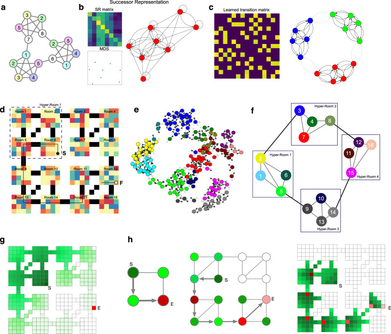
Fig. 7 CSCGs enable hierarchical abstraction and planning. The cloned graph of the CSCG lifts the observations into a hidden space, allowing for discovery of modularity that is not apparent in the visible observations. a The modular graph from8, modified to have aliased observations. Observations at each node are indicated by the numbers, and many different nodes produce the same observation. b MDS or community detection on the SR matrix of random walks in a does not reveal the modularity of the graph. c Community detection on the CSCG transition matrix successfully recovers the modularity of graph in a, recovering three communities. d A maze that has an embedded three-level hierarchy. Sensory observations are aliased both within rooms and across rooms. The black pixels denote “bridges” between the rooms. CSCG is trained on random walks from this maze. Community detection on the learned CSCG transition matrix revealed a first level of organization into rooms (e), and another level of community detection revealed hyper-rooms (f), resulting in a three-level hierarchical graph reflecting the nested structure of the maze. Planning a path (black arrows) between two rooms (denoted as (S)tart (filled black dot) and (F)inish (open black dot) in d) was achieved by finding the shortest path between hyper-rooms to navigate, next finding the shortest path between rooms, and lastly finding the shortest path within the rooms in this reduced search space. g Visualization of planning message propagation in the one-level graph. Messages propagate in the whole maze, indicating a wide search area. h Visualization of hierarchical planning. Routes are first identified on the highest level, which then becomes sub-goals at the lower level. The red colored nodes indicate the sequence of sub-goals, and their intensities reflect the ordering of the sub-goals. Compared to g, hierarchical planning requires fewer messages to be propagated so it is faster.
Fig. 7 CSCGs enable hierarchical abstraction and planning. The cloned graph of the CSCG lifts the observations into a hidden space, allowing for discovery of modularity that is not apparent in the visible observations. a The modular graph from8, modified to have aliased observations. Observations at each node are indicated by the numbers, and many different nodes produce the same observation. b MDS or community detection on the SR matrix of random walks in a does not reveal the modularity of the graph. c Community detection on the CSCG transition matrix successfully recovers the modularity of graph in a, recovering three communities. d A maze that has an embedded three-level hierarchy. Sensory observations are aliased both within rooms and across rooms. The black pixels denote “bridges” between the rooms. CSCG is trained on random walks from this maze. Community detection on the learned CSCG transition matrix revealed a first level of organization into rooms (e), and another level of community detection revealed hyper-rooms (f), resulting in a three-level hierarchical graph reflecting the nested structure of the maze. Planning a path (black arrows) between two rooms (denoted as (S)tart (filled black dot) and (F)inish (open black dot) in d) was achieved by finding the shortest path between hyper-rooms to navigate, next finding the shortest path between rooms, and lastly finding the shortest path within the rooms in this reduced search space. g Visualization of planning message propagation in the one-level graph. Messages propagate in the whole maze, indicating a wide search area. h Visualization of hierarchical planning. Routes are first identified on the highest level, which then becomes sub-goals at the lower level. The red colored nodes indicate the sequence of sub-goals, and their intensities reflect the ordering of the sub-goals. Compared to g, hierarchical planning requires fewer messages to be propagated so it is faster.CC BY · PubMed Central

Verification

Claims the paper makes

The claims and statistics of this paper haven’t been checked yet.

Free: it reads the open-access text and checks the first 5 claims that cite a source we can check. Create a free account to check every claim.

A few free checks a day · papers already verified open instantly · results are public

Claims other papers make about this one

Each is checked against this paper’s own text: does it say what the citing paper says it does?

6 more claims about this paper

Create a free account to see every claim other papers make about this one.

See all claims — free account

Self-check

Percentages, sums and reported differences re-computed from the paper’s own numbers.

The self-check needs the paper’s full text.

Citations

Cites

Show all 77 references

Research works printed but not linked: 2

  1. Whittington, J., Muller, T., Mark, S., Barry, C. & Behrens, T. Generalisation of structural knowledge in the hippocampal-entorhinal system. In Advances in Neural Information Processing Systems (eds Bengio, S. et al.) 8484–8495 (Curran Associates, Inc., 2018b).
  2. Bishop, C. M. Pattern Recognition and Machine Learning (Springer, 2006).

Cited by

See all 111

Metadata

Authors
George, D., Rikhye, R. V., Gothoskar, N., Guntupalli, J. S., Dedieu, A., & Lázaro-Gredilla, M.
Affiliations
  • Google (United States) (US)
  • Massachusetts Institute of Technology (US)
Venue
Nature Communications
Published
2021-04-22
Volume
12
Issue
1
Pages
2392-2392
ISSN
2041-1723 (ISSN-L)
OpenAlex
W3154239738
Cited by
109
References
77
Citations by year
2026: 25 · 2025: 31 · 2024: 21 · 2023: 18 · 2022: 10 · 2021: 3
FWCI
6.84
Type
journal article
Language
en
Open access
Licence
Locations
  • Nature Communications (publishedVersion, cc-by)
  • PubMed Central (publishedVersion, cc-by)
  • PubMed (publishedVersion)
  • RePEc: Research Papers in Economics (submittedVersion)
  • DOAJ (DOAJ: Directory of Open Access Journals) (submittedVersion, cc-by-sa)
Funders
  • United States Department of Defense | United States Navy | Office of Naval Research (N00014-19-1-2368)
  • Vicarious AI is a startup company and that is where the research was conducted.
Topics
  • Life Sciences › Neuroscience › Cognitive Neuroscience › Memory and Neural Mechanisms
  • Social Sciences › Psychology › Experimental and Cognitive Psychology › Spatial Cognition and Navigation
  • Life Sciences › Neuroscience › Cognitive Neuroscience › Neural dynamics and brain function
Keywords
cognitive maps, hippocampus, spatial learning, transitive inference, probabilistic sequence models, hierarchical abstraction, relational abstraction, maze navigation
MeSH terms
Cognition, Hippocampus, Humans, Learning, Markov Chains, Models, Neurological, Neural Networks, Computer

About these checks

Registry, retraction, Cites and statistics results are computed, not judged, with one exception: a printed reference that no index lists is read once by a model before it counts as a citation error. Claims are extracted by a model and kept only when their quote appears verbatim in the text; each cited source is then checked, with a model’s help, for whether it says what the claim relies on. Those verdicts can be wrong — read the claim’s quote and the cited source before relying on one.

Statistics and arithmetic are recomputed, not judged.

Confidence bands are shown only for fields calibrated on our annotated test set. None is calibrated yet, so no band is shown.

What counts as a claim ›How we measure confidence ›How we check this ›

Are you an author, or do you see a problem with this page? Request a review

How to cite

Cite CoChat for the checks on this page, and the paper for its own findings.

This page
CoChat. (2026). Citation check: Clone-structured graph representations enable flexible learning and vicarious evaluation of cognitive maps. https://app.cochat.ai/papers/10.1038/s41467-021-22559-5
The paper
George, D., Rikhye, R. V., Gothoskar, N., Guntupalli, J. S., Dedieu, A., & Lázaro-Gredilla, M. (2021). Clone-structured graph representations enable flexible learning and vicarious evaluation of cognitive maps. Nature Communications. https://doi.org/10.1038/s41467-021-22559-5

Data sources

Bibliographic data: Semantic Scholar, OpenAlex, Crossref.

Contains information from the Semantic Scholar Academic Graph Datasets, made available under the ODC Attribution License (ODC-BY 1.0).

Semantic Scholar’s data is described in: Kinney, R., et al. (2023). The Semantic Scholar Open Data Platform. arXiv:2301.10140.