Cited by 302Single-cell and spatial transcriptomicsEpigenetics and DNA MethylationGenomics and Chromatin Dynamics

The DOI matches its Crossref record; 112 of the 112 references it cites were found in a registry or an index.

DNA methylation atlas of the mouse brain at single-cell resolution

Open access

Published version of a preprint

Abstract

Abstract Mammalian brain cells show remarkable diversity in gene expression, anatomy and function, yet the regulatory DNA landscape underlying this extensive heterogeneity is poorly understood. Here we carry out a comprehensive assessment of the epigenomes of mouse brain cell types by applying single-nucleus DNA methylation sequencing 1,2 to profile 103,982 nuclei (including 95,815 neurons and 8,167 non-neuronal cells) from 45 regions of the mouse cortex, hippocampus, striatum, pallidum and olfactory areas. We identified 161 cell clusters with distinct spatial locations and projection targets. We constructed taxonomies of these epigenetic types, annotated with signature genes, regulatory elements and transcription factors. These features indicate the potential regulatory landscape supporting the assignment of putative cell types and reveal repetitive usage of regulators in excitatory and inhibitory cells for determining subtypes. The DNA methylation landscape of excitatory neurons in the cortex and hippocampus varied continuously along spatial gradients. Using this deep dataset, we constructed an artificial neural network model that precisely predicts single neuron cell-type identity and brain area spatial location. Integration of high-resolution DNA methylomes with single-nucleus chromatin accessibility data 3 enabled prediction of high-confidence enhancer–gene interactions for all identified cell types, which were subsequently validated by cell-type-specific chromatin conformation capture experiments 4 . By combining multi-omic datasets (DNA methylation, chromatin contacts, and open chromatin) from single nuclei and annotating the regulatory genome of hundreds of cell types in the mouse brain, our DNA methylation atlas establishes the epigenetic basis for neuronal diversity and spatial organization throughout the mouse cerebrum.

Overview

The claims and statistics of this paper haven’t been checked yet.

Run the check — free, no account needed. It reads the open-access text and checks the sources it cites.

A few free checks a day · papers already verified open instantly · results are public

Integrity signals

Registry

Crossref · 10.1038/s41586-020-03182-8

Cites

112 of 112 references verified0 citation errors · 0 not checkable

Statistics

Figures

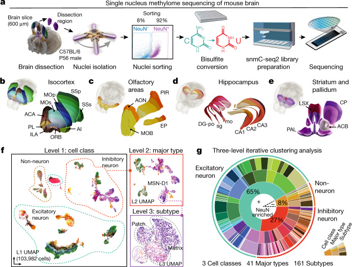
Fig. 1 A survey of single-cell DNA methylomes in the mouse brain. a, The workflow of dissection, FANS and snmC-seq2 sequencing. b–e, Dissected regions of isocortex (b), OLF (c), HIP (d) and CNU (e). f, Three-level UMAP from iterative analysis, colour coded as in b–e, panels show an example in which MSN-D1 neurons are separated into subtypes. g, Proportions of cells in clusters defined in the three-level iterative analysis. Brain atlas images in a–d were created based on Wang et al.16 and © 2017 Allen Institute for Brain Science. Allen Brain Reference Atlas. Available from: atlas.brain-map.org.
Fig. 1 A survey of single-cell DNA methylomes in the mouse brain. a, The workflow of dissection, FANS and snmC-seq2 sequencing. b–e, Dissected regions of isocortex (b), OLF (c), HIP (d) and CNU (e). f, Three-level UMAP from iterative analysis, colour coded as in b–e, panels show an example in which MSN-D1 neurons are separated into subtypes. g, Proportions of cells in clusters defined in the three-level iterative analysis. Brain atlas images in a–d were created based on Wang et al.16 and © 2017 Allen Institute for Brain Science. Allen Brain Reference Atlas. Available from: atlas.brain-map.org.CC BY · PubMed Central
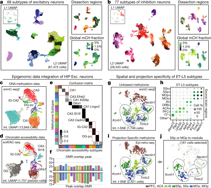
Fig. 2 Epigenomic diversity of neurons. a, b, Level 2 UMAP of excitatory (a) and inhibitory (b) neurons, coloured by subtype, dissection region and global mCH fraction. c, d, Integration UMAP of the HIP excitatory neurons profiled by snmC-seq2 (c) and snATAC-seq (d; shows pseudo-cells). e, Overlap score of a-types and m-types. f, Overlap of CG-DMR and ATAC peaks in matched subtypes. g, i, j, Integration t-SNE of ET-L5 neurons profiled by snmC-seq2 (g) and epi-retro-seq (i, j), coloured by dissection region. Three SSp- and MOp-enriched subtypes are labelled by their marker gene. j, Medulla projecting neurons from SSp or MOp only. h, Spatial composition of ET-L5 subtypes.
Fig. 2 Epigenomic diversity of neurons. a, b, Level 2 UMAP of excitatory (a) and inhibitory (b) neurons, coloured by subtype, dissection region and global mCH fraction. c, d, Integration UMAP of the HIP excitatory neurons profiled by snmC-seq2 (c) and snATAC-seq (d; shows pseudo-cells). e, Overlap score of a-types and m-types. f, Overlap of CG-DMR and ATAC peaks in matched subtypes. g, i, j, Integration t-SNE of ET-L5 neurons profiled by snmC-seq2 (g) and epi-retro-seq (i, j), coloured by dissection region. Three SSp- and MOp-enriched subtypes are labelled by their marker gene. j, Medulla projecting neurons from SSp or MOp only. h, Spatial composition of ET-L5 subtypes.CC BY · PubMed Central
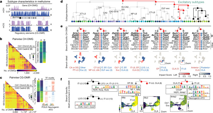
Fig. 3 Relating genes and regulatory elements to cell subtype taxonomy. a, Schematic of the two characteristics contained in the methylome profiles. b, c, Pairwise CH-DMG (b) and CG-DMR (c) counts between 68 excitatory subtypes. c, In each CG-DMR set, we further identify differentially enriched motifs (left). TF, transcription factor. d, Excitatory subtype taxonomy tree. e, Top impact scores of ranked genes for the left and right branches of nodes 1–7 in d. The top four genes are transcription factor genes (bold); these are followed by other protein-coding genes. The scatter plots below show cells involved in each branch. f, Branch-specific transcription factor motif families. The zoomed UMAPs show individual transcription factor genes in those families, whose differential mCH fractions are concordant with their motif enrichment.
Fig. 3 Relating genes and regulatory elements to cell subtype taxonomy. a, Schematic of the two characteristics contained in the methylome profiles. b, c, Pairwise CH-DMG (b) and CG-DMR (c) counts between 68 excitatory subtypes. c, In each CG-DMR set, we further identify differentially enriched motifs (left). TF, transcription factor. d, Excitatory subtype taxonomy tree. e, Top impact scores of ranked genes for the left and right branches of nodes 1–7 in d. The top four genes are transcription factor genes (bold); these are followed by other protein-coding genes. The scatter plots below show cells involved in each branch. f, Branch-specific transcription factor motif families. The zoomed UMAPs show individual transcription factor genes in those families, whose differential mCH fractions are concordant with their motif enrichment.CC BY · PubMed Central
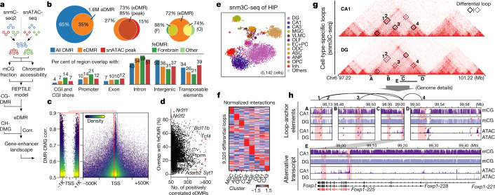
Fig. 4 Gene–enhancer landscapes in neuronal subtypes. a, Schematic of enhancer calling using matched DNA methylome and chromatin accessibility subtype profiles. Corr., correlation. b, Overlap of regulatory elements identified in this study and other epigenomic studies (ATAC peaks3 and feDMRs8). c, DMR–DMG correlation and the distance between DMR centre and gene TSS; each point is a DMR–DMG pair coloured by kernel density. d, Percentage of positively correlated eDMRs that overlap with forebrain feDMRs in each gene. e, t-SNE of cells analysed by sn-m3C-seq coloured by assigned major cell types. f, Interaction level (z-score across rows and columns) of differential loops in eight clusters at 25-kb resolution. g, h, Epigenomic signatures surrounding Foxp1. g, Triangle heat maps showing CA1 and DG chromatin contacts and differential loops. h, Genome browser sections showing detailed mCG and ATAC profiles near anchors of four CA1-specific loops. Red rectangles indicate loop anchors and red arrows indicate notable regulatory elements.
Fig. 4 Gene–enhancer landscapes in neuronal subtypes. a, Schematic of enhancer calling using matched DNA methylome and chromatin accessibility subtype profiles. Corr., correlation. b, Overlap of regulatory elements identified in this study and other epigenomic studies (ATAC peaks3 and feDMRs8). c, DMR–DMG correlation and the distance between DMR centre and gene TSS; each point is a DMR–DMG pair coloured by kernel density. d, Percentage of positively correlated eDMRs that overlap with forebrain feDMRs in each gene. e, t-SNE of cells analysed by sn-m3C-seq coloured by assigned major cell types. f, Interaction level (z-score across rows and columns) of differential loops in eight clusters at 25-kb resolution. g, h, Epigenomic signatures surrounding Foxp1. g, Triangle heat maps showing CA1 and DG chromatin contacts and differential loops. h, Genome browser sections showing detailed mCG and ATAC profiles near anchors of four CA1-specific loops. Red rectangles indicate loop anchors and red arrows indicate notable regulatory elements.CC BY · PubMed Central
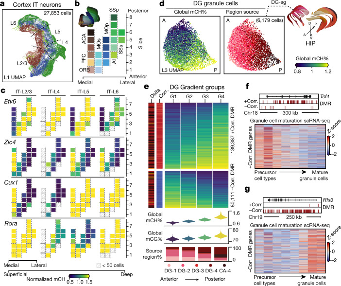
Fig. 5 Brain-wide spatial gradients of DNA methylation. a, UMAP for cortex IT neurons coloured by dissection regions. b, The 21 cortical dissection regions organized by spatial axis. c, Normalized mCH fraction of spatial CH-DMGs, with the same layout as b. d, UMAPs for DG granule cells coloured by their cell global mCH fractions and dissection regions. A, anterior; P, posterior; D, dorsal; V, ventral. e, Compound figure showing four cells groups organized according to DG gradient and the two gradient DMR groups separated according to the sign of the correlation to the cell’s global mCH level. f, g, Bottom, expression (z-score across rows) of genes positively (f) or negatively (g) correlated with DMRs across cell types along the granule cell maturation pathway33. Top, genome browser views of representative genes.
Fig. 5 Brain-wide spatial gradients of DNA methylation. a, UMAP for cortex IT neurons coloured by dissection regions. b, The 21 cortical dissection regions organized by spatial axis. c, Normalized mCH fraction of spatial CH-DMGs, with the same layout as b. d, UMAPs for DG granule cells coloured by their cell global mCH fractions and dissection regions. A, anterior; P, posterior; D, dorsal; V, ventral. e, Compound figure showing four cells groups organized according to DG gradient and the two gradient DMR groups separated according to the sign of the correlation to the cell’s global mCH level. f, g, Bottom, expression (z-score across rows) of genes positively (f) or negatively (g) correlated with DMRs across cell types along the granule cell maturation pathway33. Top, genome browser views of representative genes.CC BY · PubMed Central
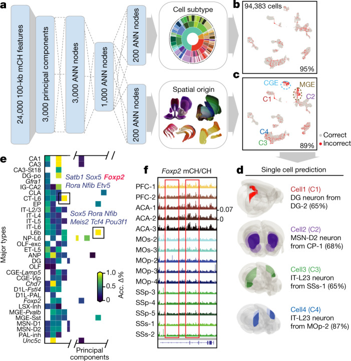
Fig. 6 A methylome-based predictive model captures both cellular and spatial characteristics of neurons. a, Schematic of the model that predicts both cell-type identity and spatial origin. b, c, Model performance on the prediction of cell subtypes (b), and dissection regions (c). Per cent accuracy is shown. d, Examples of using the model to predict cell spatial origin (maximum prediction probability in parentheses). e, Evaluation of importance of features (principal components) for spatial origin prediction accuracy. ‘Acc. Δ%’ denotes the average prediction accuracy decrease percentage. f, The Foxp2 gene body mCH fraction in each cortical dissection region group.
Fig. 6 A methylome-based predictive model captures both cellular and spatial characteristics of neurons. a, Schematic of the model that predicts both cell-type identity and spatial origin. b, c, Model performance on the prediction of cell subtypes (b), and dissection regions (c). Per cent accuracy is shown. d, Examples of using the model to predict cell spatial origin (maximum prediction probability in parentheses). e, Evaluation of importance of features (principal components) for spatial origin prediction accuracy. ‘Acc. Δ%’ denotes the average prediction accuracy decrease percentage. f, The Foxp2 gene body mCH fraction in each cortical dissection region group.CC BY · PubMed Central
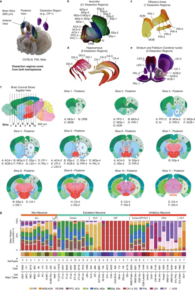
Extended Data Fig. 1 Brain dissection regions. a, Schematic of brain dissection steps. Each male C57BL/6 mouse brain (age P56) was dissected into 600-μm slices. We then dissected brain regions from both hemispheres within a specific slice. b–e, 3D mouse brain schematic adapted from Allen CCFv3 to display the four major brain regions and 45 dissection regions. Each colour represents a dissection region. f, 2D mouse brain atlas adapted from Allen Mouse Brain Reference Atlas, the first sagittal image showing the location of each coronal slice, followed by 11 posterior view images of all coronal slices, the same 45 dissection regions are labelled on the corresponding slice. All coronal images follow the same scale as the sagittal image. The posterior view of each slice is the anterior view of the next slice. g, An integrated overview of brain region composition, subtype and cell numbers of the major types. All brain atlas images were created based on Wang et al.16 and © 2017 Allen Institute for Brain Science. Allen Brain Reference Atlas. Available from: http://www.atlas.brain-map.org.
Extended Data Fig. 1 Brain dissection regions. a, Schematic of brain dissection steps. Each male C57BL/6 mouse brain (age P56) was dissected into 600-μm slices. We then dissected brain regions from both hemispheres within a specific slice. b–e, 3D mouse brain schematic adapted from Allen CCFv3 to display the four major brain regions and 45 dissection regions. Each colour represents a dissection region. f, 2D mouse brain atlas adapted from Allen Mouse Brain Reference Atlas, the first sagittal image showing the location of each coronal slice, followed by 11 posterior view images of all coronal slices, the same 45 dissection regions are labelled on the corresponding slice. All coronal images follow the same scale as the sagittal image. The posterior view of each slice is the anterior view of the next slice. g, An integrated overview of brain region composition, subtype and cell numbers of the major types. All brain atlas images were created based on Wang et al.16 and © 2017 Allen Institute for Brain Science. Allen Brain Reference Atlas. Available from: http://www.atlas.brain-map.org.CC BY · PubMed Central
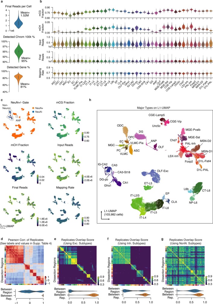
Extended Data Fig. 2 Major Type labelling and basic mapping metrics of snmC-seq2. a, The number of final pass QC reads, the percentage of non-overlapping chromosome 100-kb bins detected, and the percentage of GENCODE vm22 genes detected per cell. b, Violin plots for all of the key metrics, group by major types. c, L1 UMAP coloured by NeuN antibody FACS gates and other snmC-seq2 key read mapping metrics. d, Heat map of Pearson correlation between the average methylome profiles (mean mCH and mCG fraction of all chromosome 100-kb bins across all cells belong to a replicate sample) of the 92 replicates from 45 brain regions. The violin plot below summarizes the value between replicates within the same brain region or between different brain regions. e–g, Pairwise overlap score (measuring co-clustering of two replicates) of excitatory subtypes (e), inhibitory subtypes (f), and non-neuronal subtypes (g). The violin plots summarize the subtype overlap score between replicates within the same brain region or between different brain regions. h, L1 UMAP coloured and labelled by major cell types.
Extended Data Fig. 2 Major Type labelling and basic mapping metrics of snmC-seq2. a, The number of final pass QC reads, the percentage of non-overlapping chromosome 100-kb bins detected, and the percentage of GENCODE vm22 genes detected per cell. b, Violin plots for all of the key metrics, group by major types. c, L1 UMAP coloured by NeuN antibody FACS gates and other snmC-seq2 key read mapping metrics. d, Heat map of Pearson correlation between the average methylome profiles (mean mCH and mCG fraction of all chromosome 100-kb bins across all cells belong to a replicate sample) of the 92 replicates from 45 brain regions. The violin plot below summarizes the value between replicates within the same brain region or between different brain regions. e–g, Pairwise overlap score (measuring co-clustering of two replicates) of excitatory subtypes (e), inhibitory subtypes (f), and non-neuronal subtypes (g). The violin plots summarize the subtype overlap score between replicates within the same brain region or between different brain regions. h, L1 UMAP coloured and labelled by major cell types.CC BY · PubMed Central
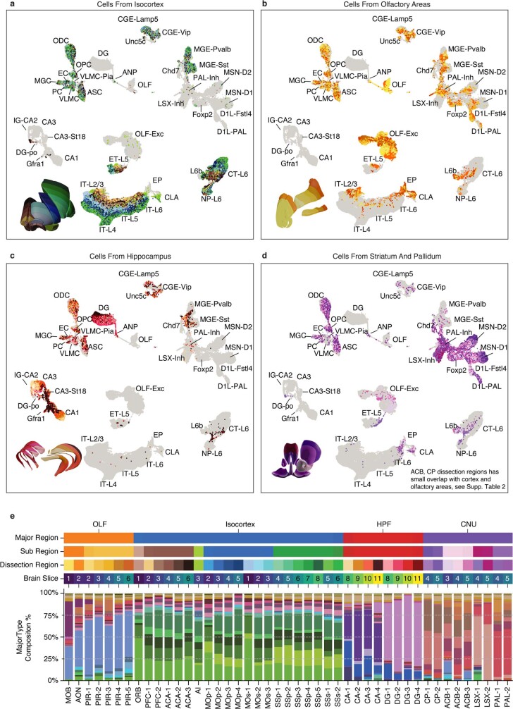
Extended Data Fig. 3 Cell-type composition of dissection regions. a-d, L1 UMAP labelled by major types and partially coloured by dissection regions for cells from isocortex (a), OLF (b), HIP (c) and cerebral nucleus (d). Other cells are shown in grey as background. e, Similar compound bar plot as Extended Data Fig. 1g, arranged top to bottom, showing the organization of dissection regions and the major type composition of each dissection region.
Extended Data Fig. 3 Cell-type composition of dissection regions. a-d, L1 UMAP labelled by major types and partially coloured by dissection regions for cells from isocortex (a), OLF (b), HIP (c) and cerebral nucleus (d). Other cells are shown in grey as background. e, Similar compound bar plot as Extended Data Fig. 1g, arranged top to bottom, showing the organization of dissection regions and the major type composition of each dissection region.CC BY · PubMed Central
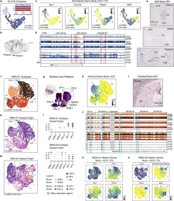
Extended Data Fig. 4 Supporting details of cellular and spatial diversity of neurons at the subtype level. a, Level 3 UMAP of IG-CA2 neurons coloured by subtypes. Bar plot showing sub-region composition of the subtypes: (1) Xpr1, (2) Chrm3, and (3) Peak1. b, The 3D model illustrates the spatial relationships between related anatomical structures. c, mCH fraction of marker genes in IG-CA2 cells. d, Methylome, and chromatin accessibility genome browser view of Ntf3 genes and its upstream regions. ATAC and eDMR information are from Fig. 4 analysis. e, Three different views of the in situ hybridization experiment (source: https://mouse.brain-map.org/gene/show/17972; the same patterns were shown in three biological replicates) from Allen Brain Atlas48, showing the Ntf3 gene expressed in both IG and CA2. f, Level 3 UMAP of MSN-D1 neurons coloured by subtype. Numbers indicate four subtypes: (1) Khdrbs3, (2) Hrh1 (3) Plxnc1, and (4) Ntn1. g, The 3D model of related striatum dissection regions. h, i, mCH fraction (h), and an in situ hybridization experiment (source: https://mouse.brain-map.org/gene/show/13769; the same patterns were shown in two biological replicates) from Allen Brain Atlas48 (i) of the Khdrbs3 gene, red arrows indicate patch regions in CP. j, Genome browser view of Khdrbs3 genes similar to d. k, Level 3 UMAP of MSN-D1 neurons coloured by dissection regions. l, The region composition of each subtype of MSN-D1 and MSN-D2. m, MSN-D2 subtypes: (1) Nrp2, (2) Casz1, (3) Col14a1, and (4) Slc24a2. n, o, mCH fraction of MSN-D1 (n) and MSN-D2 (o) subtype marker genes. All brain atlas images (b, g) were created based on Wang et al.16 and © 2017 Allen Institute for Brain Science. Allen Brain Reference Atlas. Available from: http://atlas.brain-map.org.
Extended Data Fig. 4 Supporting details of cellular and spatial diversity of neurons at the subtype level. a, Level 3 UMAP of IG-CA2 neurons coloured by subtypes. Bar plot showing sub-region composition of the subtypes: (1) Xpr1, (2) Chrm3, and (3) Peak1. b, The 3D model illustrates the spatial relationships between related anatomical structures. c, mCH fraction of marker genes in IG-CA2 cells. d, Methylome, and chromatin accessibility genome browser view of Ntf3 genes and its upstream regions. ATAC and eDMR information are from Fig. 4 analysis. e, Three different views of the in situ hybridization experiment (source: https://mouse.brain-map.org/gene/show/17972; the same patterns were shown in three biological replicates) from Allen Brain Atlas48, showing the Ntf3 gene expressed in both IG and CA2. f, Level 3 UMAP of MSN-D1 neurons coloured by subtype. Numbers indicate four subtypes: (1) Khdrbs3, (2) Hrh1 (3) Plxnc1, and (4) Ntn1. g, The 3D model of related striatum dissection regions. h, i, mCH fraction (h), and an in situ hybridization experiment (source: https://mouse.brain-map.org/gene/show/13769; the same patterns were shown in two biological replicates) from Allen Brain Atlas48 (i) of the Khdrbs3 gene, red arrows indicate patch regions in CP. j, Genome browser view of Khdrbs3 genes similar to d. k, Level 3 UMAP of MSN-D1 neurons coloured by dissection regions. l, The region composition of each subtype of MSN-D1 and MSN-D2. m, MSN-D2 subtypes: (1) Nrp2, (2) Casz1, (3) Col14a1, and (4) Slc24a2. n, o, mCH fraction of MSN-D1 (n) and MSN-D2 (o) subtype marker genes. All brain atlas images (b, g) were created based on Wang et al.16 and © 2017 Allen Institute for Brain Science. Allen Brain Reference Atlas. Available from: http://atlas.brain-map.org.CC BY · PubMed Central
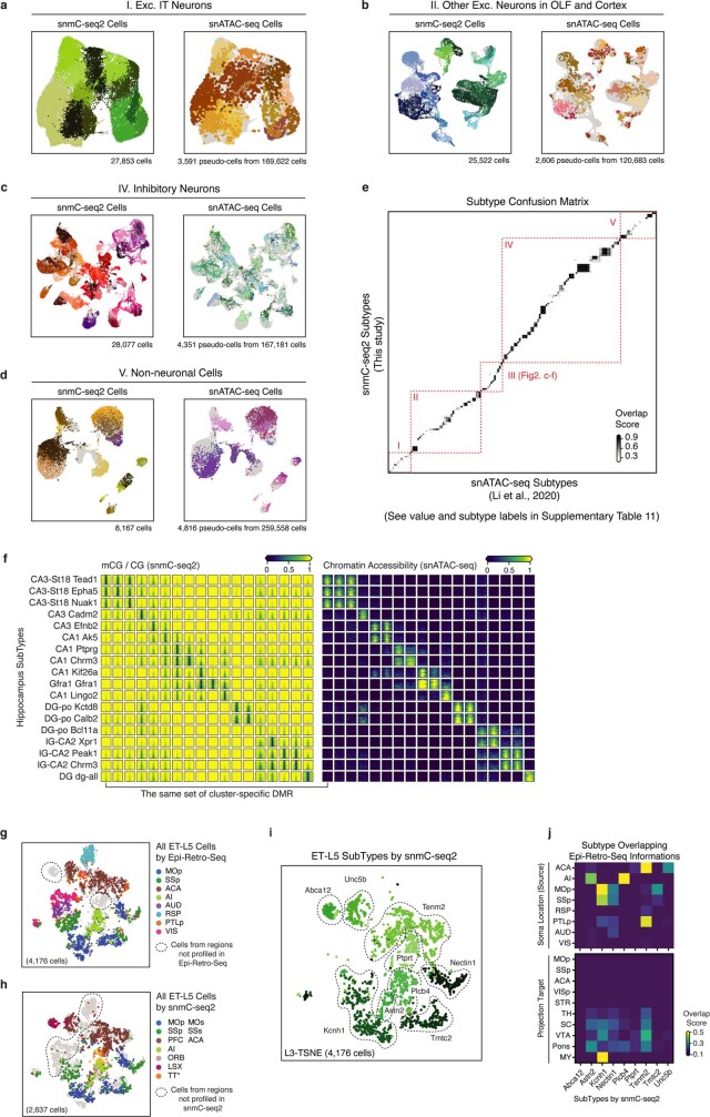
Extended Data Fig. 5 Integration with snATAC-seq and epi-retro-seq. a–d, Integration UMAP for snmC-seq2 cells and snATAC-seq pseudo-cells from each cell group: excitatory IT neurons (a), other excitatory neurons (b), inhibitory neurons (c) and non-neuronal cells (d). Each panel is coloured by subtypes from the corresponding study, the other dataset is shown in grey in the background. e, Overlap score matrix matching the 160 a-types to the 161 m-types. f, mCG fraction (left), and chromatin accessibility (right) of cluster-specific CG-DMRs (columns) in HIP subtypes (rows). g, h, Same integration t-SNE as Fig. 2g, i coloured by the dissection regions but using all cells profiled by epi-retro-seq (g) or snmC-seq2 (h), cells from brain regions that have only been profiled via one of the methods are circled out. i, Same t-SNE as (h) coloured by snmC-seq2 subtypes. j, Overlap score matrix matching the subtypes to the ‘Soma Location (source)’ and ‘Projection target’ information labels of epi-retro-seq cells.
Extended Data Fig. 5 Integration with snATAC-seq and epi-retro-seq. a–d, Integration UMAP for snmC-seq2 cells and snATAC-seq pseudo-cells from each cell group: excitatory IT neurons (a), other excitatory neurons (b), inhibitory neurons (c) and non-neuronal cells (d). Each panel is coloured by subtypes from the corresponding study, the other dataset is shown in grey in the background. e, Overlap score matrix matching the 160 a-types to the 161 m-types. f, mCG fraction (left), and chromatin accessibility (right) of cluster-specific CG-DMRs (columns) in HIP subtypes (rows). g, h, Same integration t-SNE as Fig. 2g, i coloured by the dissection regions but using all cells profiled by epi-retro-seq (g) or snmC-seq2 (h), cells from brain regions that have only been profiled via one of the methods are circled out. i, Same t-SNE as (h) coloured by snmC-seq2 subtypes. j, Overlap score matrix matching the subtypes to the ‘Soma Location (source)’ and ‘Projection target’ information labels of epi-retro-seq cells.CC BY · PubMed Central
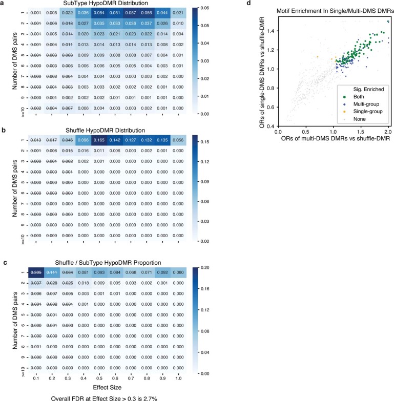
Extended Data Fig. 6 Controlling the FDR of CG-DMRs. a, b, The proportion of subtype (a) or shuffled DMRs (b) in each block of specific effect size and number of DMSs. c, The empirical FDR of each block, calculated by (no. of shuffle-DMRs/no. of subtype-DMRs) in each block. DMRs with effect size <0.3 were excluded in further analyses. d, The odds ratio of transcription factor motif enrichment in single-DMS DMRs (sDMRs) and multi-DMS DMRs (mDMRs). Each dot represents a transcription factor. Transcription factors whose motifs are significantly enriched in both sDMRs and mDMRs are coloured in green, and transcription factors that are significant only in sDMR or mDMRs are coloured in red or blue, respectively. Non-significant transcription factors are shown in grey.
Extended Data Fig. 6 Controlling the FDR of CG-DMRs. a, b, The proportion of subtype (a) or shuffled DMRs (b) in each block of specific effect size and number of DMSs. c, The empirical FDR of each block, calculated by (no. of shuffle-DMRs/no. of subtype-DMRs) in each block. DMRs with effect size <0.3 were excluded in further analyses. d, The odds ratio of transcription factor motif enrichment in single-DMS DMRs (sDMRs) and multi-DMS DMRs (mDMRs). Each dot represents a transcription factor. Transcription factors whose motifs are significantly enriched in both sDMRs and mDMRs are coloured in green, and transcription factors that are significant only in sDMR or mDMRs are coloured in red or blue, respectively. Non-significant transcription factors are shown in grey.CC BY · PubMed Central
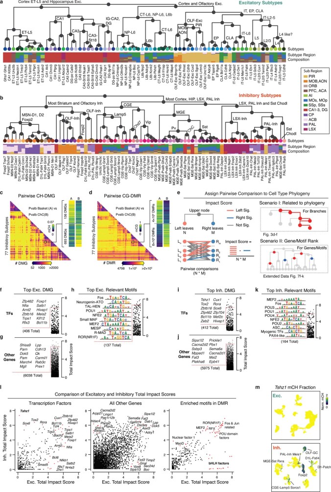
Extended Data Fig. 7 Subtype taxonomy with related genes and motifs. a, b, Subtype taxonomy of excitatory (a) and inhibitory (b) neurons. Leaf nodes are coloured by subtypes, and the bar plot shows subregion composition. c, d, Counts heat map of pairwise CH-DMG (c) and CG-DMR (d) between 77 inhibitory subtypes. e, Schematic of impact score calculation (left), and two scenarios of discussing impact scores (right). f–h, Top transcription factors (f), other genes (g) and enriched motifs (h) ranked by total impact score based on the excitatory subtype taxonomy. i–k, Top transcription factors (i), other genes (j) and enriched motifs (k) ranked by total impact score based on the inhibitory subtype taxonomy. l, Comparison of the total impact scores calculated from either excitatory subtype taxonomy (x-axis) or inhibitory subtype taxonomy (y-axis) for transcription factors, other genes and enriched motifs. m, An example gene Tshz1 only shows subtype diversity in inhibitory subtypes but not in excitatory subtypes.
Extended Data Fig. 7 Subtype taxonomy with related genes and motifs. a, b, Subtype taxonomy of excitatory (a) and inhibitory (b) neurons. Leaf nodes are coloured by subtypes, and the bar plot shows subregion composition. c, d, Counts heat map of pairwise CH-DMG (c) and CG-DMR (d) between 77 inhibitory subtypes. e, Schematic of impact score calculation (left), and two scenarios of discussing impact scores (right). f–h, Top transcription factors (f), other genes (g) and enriched motifs (h) ranked by total impact score based on the excitatory subtype taxonomy. i–k, Top transcription factors (i), other genes (j) and enriched motifs (k) ranked by total impact score based on the inhibitory subtype taxonomy. l, Comparison of the total impact scores calculated from either excitatory subtype taxonomy (x-axis) or inhibitory subtype taxonomy (y-axis) for transcription factors, other genes and enriched motifs. m, An example gene Tshz1 only shows subtype diversity in inhibitory subtypes but not in excitatory subtypes.CC BY · PubMed Central
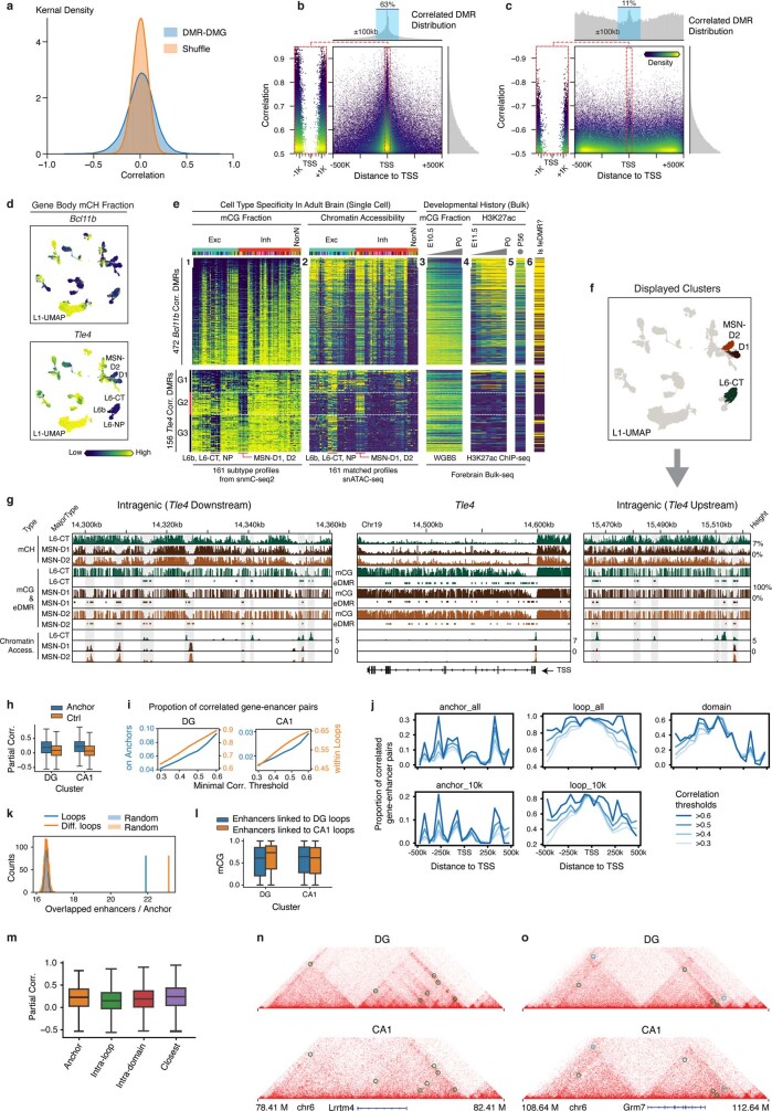
Extended Data Fig. 8 Gene-Enhancer landscape related. a, Distribution of actual DMR–DMG partial correlation compared to the shuffled null distribution. b, c, DMR–DMG correlation (y-axis), and the distance between DMR centre and gene TSS (x-axis), each point is a DMR–DMG pair, colour represents points kernel density. The positively (b) and negatively (c) correlated DMRs are shown separately, owing to very different genome location distributions that are plotted on the top histograms. d, The gene body mCH fraction of Bcl11b (top) and Tle4 (bottom) gene. e, The predicted enhancer landscape of Bcl11b (top) and Tle4 (bottom). Each row is a correlated eDMR to the gene, columns from left to right are: (1) mCG fraction and (2) ATAC FPKM in 161 subtypes; (3) bulk developing forebrain tissue mCG fraction and (4) H3K27ac FPKM; (5) adult frontal cortex H3K27ac FPKM; and (6) feDMR or not. f, detailed view of surrounding eDMRs that are correlated with Tle4 gene body mCH. Alternative eDMRs appear only in either CT-L6 or MSN-D1/D2 can be seen both upstream and downstream of the gene. g, Level 1 UMAP coloured by corresponding cell major types shown in f. h, Partial correlation between mCG of enhancers and mCH of genes on separated loop anchors of DG (left) and CA1 (right) compared to random anchors with comparable distance (n = 4,171, 4,036, 4,326, 5,133 (left to right)), P = 5.9 × 10−74 for DG and 3.0 × 10−158 for CA1, two-sided Wilcoxon rank-sum tests. i, Proportion of loop supported enhancer-gene pairs among the pairs linked by correlation analyses surpassing different correlation thresholds in DG (left) and CA1 (right). The proportion of pairs that the gene and enhancer located on separated anchors of the same loop (blue, left y-axis) or within the same loop (orange, right y-axis) is shown. j, Proportion of loop supported enhancer-gene pairs among those linked by correlation analyses surpassing different correlation thresholds at each specific distance. k, Number of enhancers per loop anchor (blue) or per differential loop anchor (orange) compared to randomly selected 25-kb regions across the genome.; P < 0.005, two-sided permutation test with 2,000 times repeats. l, mCG of enhancers linking to DG specific loops (blue, n = 13,854) and CA1-specific loops (orange, n = 14,373) in DG (left, P = 2.9× 10⁻³) or CA1 (right, P = 3.5 × 10⁻⁵). P values were computed with two-sided Wilcoxon rank-sum tests. m, Partial correlation between mCG of enhancers and mCH of genes linked by different methods (n = 4,171, 127,730, 28,203, 10,058 (left to right)). The elements of box plots are defined as: centre line, median; box limits, first and third quartiles; whiskers, 1.5 × interquartile range. n, o, Interaction maps, mCH, mCG, ATAC and differential loops tracks surrounding Lrrtm4 (n) and Grm7 (o). Circles on the interaction maps represent differential loops between DG and CA1, where green represents DG loops, and cyan represents CA1 loops.
Extended Data Fig. 8 Gene-Enhancer landscape related. a, Distribution of actual DMR–DMG partial correlation compared to the shuffled null distribution. b, c, DMR–DMG correlation (y-axis), and the distance between DMR centre and gene TSS (x-axis), each point is a DMR–DMG pair, colour represents points kernel density. The positively (b) and negatively (c) correlated DMRs are shown separately, owing to very different genome location distributions that are plotted on the top histograms. d, The gene body mCH fraction of Bcl11b (top) and Tle4 (bottom) gene. e, The predicted enhancer landscape of Bcl11b (top) and Tle4 (bottom). Each row is a correlated eDMR to the gene, columns from left to right are: (1) mCG fraction and (2) ATAC FPKM in 161 subtypes; (3) bulk developing forebrain tissue mCG fraction and (4) H3K27ac FPKM; (5) adult frontal cortex H3K27ac FPKM; and (6) feDMR or not. f, detailed view of surrounding eDMRs that are correlated with Tle4 gene body mCH. Alternative eDMRs appear only in either CT-L6 or MSN-D1/D2 can be seen both upstream and downstream of the gene. g, Level 1 UMAP coloured by corresponding cell major types shown in f. h, Partial correlation between mCG of enhancers and mCH of genes on separated loop anchors of DG (left) and CA1 (right) compared to random anchors with comparable distance (n = 4,171, 4,036, 4,326, 5,133 (left to right)), P = 5.9 × 10−74 for DG and 3.0 × 10−158 for CA1, two-sided Wilcoxon rank-sum tests. i, Proportion of loop supported enhancer-gene pairs among the pairs linked by correlation analyses surpassing different correlation thresholds in DG (left) and CA1 (right). The proportion of pairs that the gene and enhancer located on separated anchors of the same loop (blue, left y-axis) or within the same loop (orange, right y-axis) is shown. j, Proportion of loop supported enhancer-gene pairs among those linked by correlation analyses surpassing different correlation thresholds at each specific distance. k, Number of enhancers per loop anchor (blue) or per differential loop anchor (orange) compared to randomly selected 25-kb regions across the genome.; P < 0.005, two-sided permutation test with 2,000 times repeats. l, mCG of enhancers linking to DG specific loops (blue, n = 13,854) and CA1-specific loops (orange, n = 14,373) in DG (left, P = 2.9× 10⁻³) or CA1 (right, P = 3.5 × 10⁻⁵). P values were computed with two-sided Wilcoxon rank-sum tests. m, Partial correlation between mCG of enhancers and mCH of genes linked by different methods (n = 4,171, 127,730, 28,203, 10,058 (left to right)). The elements of box plots are defined as: centre line, median; box limits, first and third quartiles; whiskers, 1.5 × interquartile range. n, o, Interaction maps, mCH, mCG, ATAC and differential loops tracks surrounding Lrrtm4 (n) and Grm7 (o). Circles on the interaction maps represent differential loops between DG and CA1, where green represents DG loops, and cyan represents CA1 loops.CC BY · PubMed Central
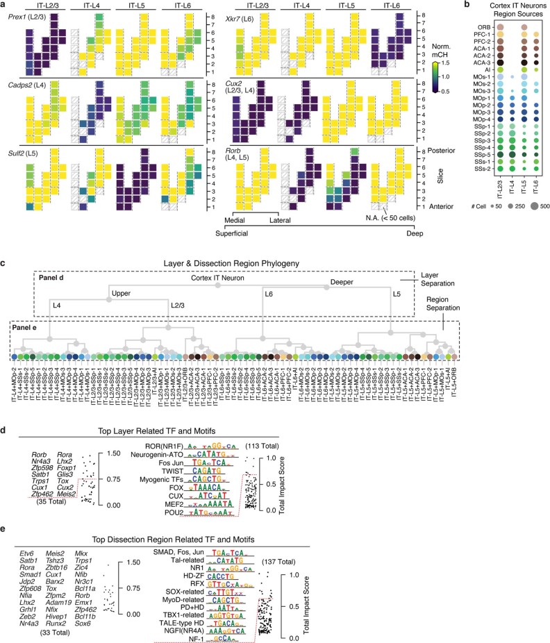
Extended Data Fig. 9 DNA methylation gradient of IT neurons. a, Representative marker genes for laminar layers separation. The same dissection region layout in Fig. 5b was used here. b, Layer-dissection-region cell group taxonomy. c, Dot plot sized by the number of cells in each layer-dissection-region combination in excitatory IT neurons. Each group needs at least 50 cells to be included in the analysis. d, e, The top layer (d) and dissection region (e) for related TFs and JASPAR motifs ranked by total impact score.
Extended Data Fig. 9 DNA methylation gradient of IT neurons. a, Representative marker genes for laminar layers separation. The same dissection region layout in Fig. 5b was used here. b, Layer-dissection-region cell group taxonomy. c, Dot plot sized by the number of cells in each layer-dissection-region combination in excitatory IT neurons. Each group needs at least 50 cells to be included in the analysis. d, e, The top layer (d) and dissection region (e) for related TFs and JASPAR motifs ranked by total impact score.CC BY · PubMed Central
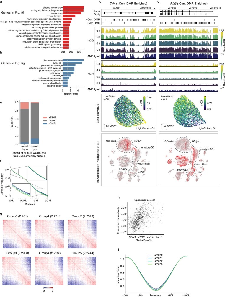
Extended Data Fig. 10 DNA methylation gradient of DG granule cells. a, b, Top enriched Gene Ontology (GO) terms for +DMRgenes (a) and −DMRgenes (b). Significant +DMRgenes and −DMRgenes are coloured in red and blue, respectively. c, d, For the +DMRgene Tcf4 (c) or the −DMRgene Rfx3 (d), the browser view of +DMRs or −DMRs, mCG or mCH in each DG cells groups and adult neural progenitors (ANP), L3 UMAP coloured by gene body mCG, and scRNA-Seq UMAP coloured by gene expression are shown. e, The proportion of dorsal or ventral DMRs that overlap with +DMRs and −DMRs. f, Interaction frequency decays with increasing genome distances in different groups. g, Saddle plots for different groups of DG cells separated by global mCH. Values in the title represent the compartment’s strengths. h, Correlation between global mCH and proportion of intra-domain contacts across 1,904 DG cells. i, Insulation scores of 9,160 domain boundaries and flanking 100-kb regions.
Extended Data Fig. 10 DNA methylation gradient of DG granule cells. a, b, Top enriched Gene Ontology (GO) terms for +DMRgenes (a) and −DMRgenes (b). Significant +DMRgenes and −DMRgenes are coloured in red and blue, respectively. c, d, For the +DMRgene Tcf4 (c) or the −DMRgene Rfx3 (d), the browser view of +DMRs or −DMRs, mCG or mCH in each DG cells groups and adult neural progenitors (ANP), L3 UMAP coloured by gene body mCG, and scRNA-Seq UMAP coloured by gene expression are shown. e, The proportion of dorsal or ventral DMRs that overlap with +DMRs and −DMRs. f, Interaction frequency decays with increasing genome distances in different groups. g, Saddle plots for different groups of DG cells separated by global mCH. Values in the title represent the compartment’s strengths. h, Correlation between global mCH and proportion of intra-domain contacts across 1,904 DG cells. i, Insulation scores of 9,160 domain boundaries and flanking 100-kb regions.CC BY · PubMed Central
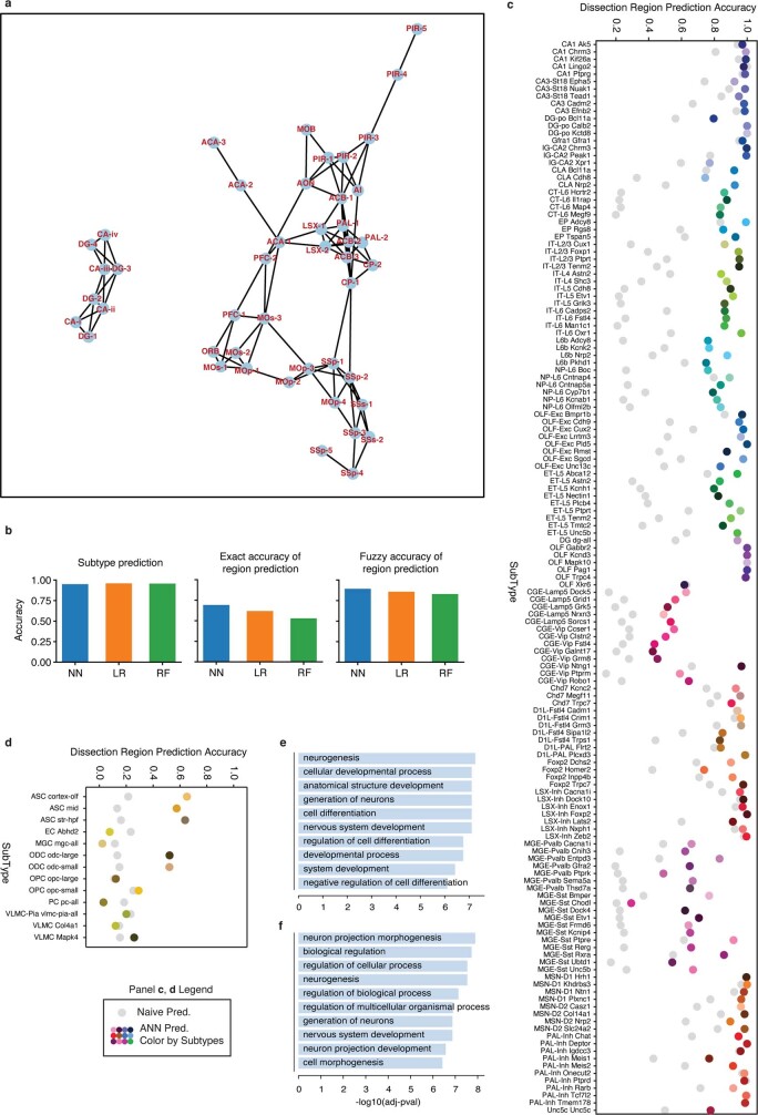
Extended Data Fig. 11 Evaluation of the predictive model. a, The neighbour relation among the potential overlapping dissection regions. The network is constructed based on information of the dissection scheme and the ‘Potential overlap’ column in Supplementary Table 2 and is used to compute the fuzzy accuracy. b, The exact accuracy of subtype prediction (top), dissected region prediction (middle), and fuzzy accuracy of dissected region prediction (bottom) of neural network (NN, blue), logistic regression (LR, orange) and random forest (RF, green). c, d, Prediction accuracy of dissection region at cell subtype level of neurons (c) and non-neuronal cells (d). Coloured points denote the prediction accuracy of the model, whereas grey points denote the random guess accuracy when cell subtypes and corresponding spatial distributions are given. g, h, GO-term enrichment of top-loading genes of features that are important for predicting the spatial location of CT-L6 (g) and L6b (h).
Extended Data Fig. 11 Evaluation of the predictive model. a, The neighbour relation among the potential overlapping dissection regions. The network is constructed based on information of the dissection scheme and the ‘Potential overlap’ column in Supplementary Table 2 and is used to compute the fuzzy accuracy. b, The exact accuracy of subtype prediction (top), dissected region prediction (middle), and fuzzy accuracy of dissected region prediction (bottom) of neural network (NN, blue), logistic regression (LR, orange) and random forest (RF, green). c, d, Prediction accuracy of dissection region at cell subtype level of neurons (c) and non-neuronal cells (d). Coloured points denote the prediction accuracy of the model, whereas grey points denote the random guess accuracy when cell subtypes and corresponding spatial distributions are given. g, h, GO-term enrichment of top-loading genes of features that are important for predicting the spatial location of CT-L6 (g) and L6b (h).CC BY · PubMed Central

Verification

Claims the paper makes

The claims and statistics of this paper haven’t been checked yet.

Run the check — free, no account needed. It reads the open-access text and checks the sources it cites.

A few free checks a day · papers already verified open instantly · results are public

Claims other papers make about this one

Each is checked against this paper’s own text: does it say what the citing paper says it does?

Self-check

Percentages, sums and reported differences re-computed from the paper’s own numbers.

The self-check needs the paper’s full text.

Citations

Cites

Show all 102 references

Cited by

Sorted by citations

See all 302

Metadata

Authors
Liu, H., Zhou, J., Tian, W., Luo, C., Bartlett, A., Aldridge, A., Lucero, J., Osteen, J. K., Nery, J. R., Chen, H., Rivkin, A., Castanon, R. G., Clock, B., Li, Y. E., Hou, X., Poirion, O. B., Preissl, S., Pinto-Duarte, A., O’Connor, C., Boggeman, L., Fitzpatrick, C., Nunn, M., Mukamel, E. A., Zhang, Z., Callaway, E. M., Ren, B., Dixon, J. R., Behrens, M. M., & Ecker, J. R.
Affiliations
  • Salk Institute for Biological Studies (US)
  • Ludwig Cancer Research (US)
  • University of California San Diego (US)
Corresponding author
Ecker, Joseph R.
Venue
Nature
Published
2021-10-06
Volume
598
Issue
7879
Pages
120-128
ISSN
  • 0028-0836 (ISSN-L)
  • 1476-4687
OpenAlex
W3203959602
Cited by
289
References
102
Citations by year
2026: 50 · 2025: 66 · 2024: 59 · 2023: 52 · 2022: 46 · 2021: 14
FWCI
14.21
Type
journal article
Language
en
Open access
Locations
  • Nature (publishedVersion, cc-by)
  • bioRxiv (Cold Spring Harbor Laboratory) (acceptedVersion, cc-by-nc-nd)
  • PubMed Central (publishedVersion, cc-by)
  • PubMed (publishedVersion)
  • RePEc: Research Papers in Economics (submittedVersion)
  • eScholarship (California Digital Library) (submittedVersion)
  • eScholarship (California Digital Library) (submittedVersion, cc-by)
  • FreiDok plus (Universitätsbibliothek Freiburg) (submittedVersion)
Funders
  • Howard Hughes Medical Institute
  • National Institutes of Health (NCI CCSG: P30 014195, P30 014195, 1s10od023689-01a1)
  • National Institute of Mental Health (U19MH114831, U19MH114830, F30MH011483)
  • National Human Genome Research Institute (R01HG010634)
  • National Cancer Institute (S10-OD023689, CCSG:P30 014195, NIH-NCI CCSG: P30 014195, P30014195, P30CA014195)
Topics
  • Life Sciences › Biochemistry, Genetics and Molecular Biology › Molecular Biology › Single-cell and spatial transcriptomics
  • Life Sciences › Biochemistry, Genetics and Molecular Biology › Molecular Biology › Epigenetics and DNA Methylation
  • Life Sciences › Biochemistry, Genetics and Molecular Biology › Molecular Biology › Genomics and Chromatin Dynamics
Keywords
DNA methylation, mouse brain, neuronal cell types, excitatory and inhibitory neurons, enhancer-gene interactions, chromatin accessibility, hippocampus, cerebral cortex, olfactory bulb, striatum, globus pallidus, transcription factors, regulatory elements
MeSH terms
Epigenome, Animals, Atlases as Topic, Brain, Chromatin, Cytosine, Enhancer Elements, Genetic, Hippocampus, Male, Mice, Inbred C57BL, Models, Biological, Neural Pathways, Neurons, Dentate Gyrus, DNA Methylation, Gene Expression Profiling, Mice, Epigenomics, Single-Cell Analysis, Datasets as Topic

About these checks

Registry, retraction, Cites and statistics results are computed, not judged, with one exception: a printed reference that no index lists is read once by a model before it counts as a citation error. Claims are extracted by a model and kept only when their quote appears verbatim in the text; each cited source is then checked, with a model’s help, for whether it says what the claim relies on. Those verdicts can be wrong — read the claim’s quote and the cited source before relying on one.

Statistics and arithmetic are recomputed, not judged.

Confidence bands are shown only for fields calibrated on our annotated test set. None is calibrated yet, so no band is shown.

What counts as a claim ›How we measure confidence ›How we check this ›

Are you an author, or do you see a problem with this page? Request a review