

The DOI matches its Crossref record; 29 of the 29 references it cites were found in a registry or an index.
LIVECell—A large-scale dataset for label-free live cell segmentation
Open accessAbstract
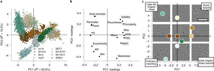
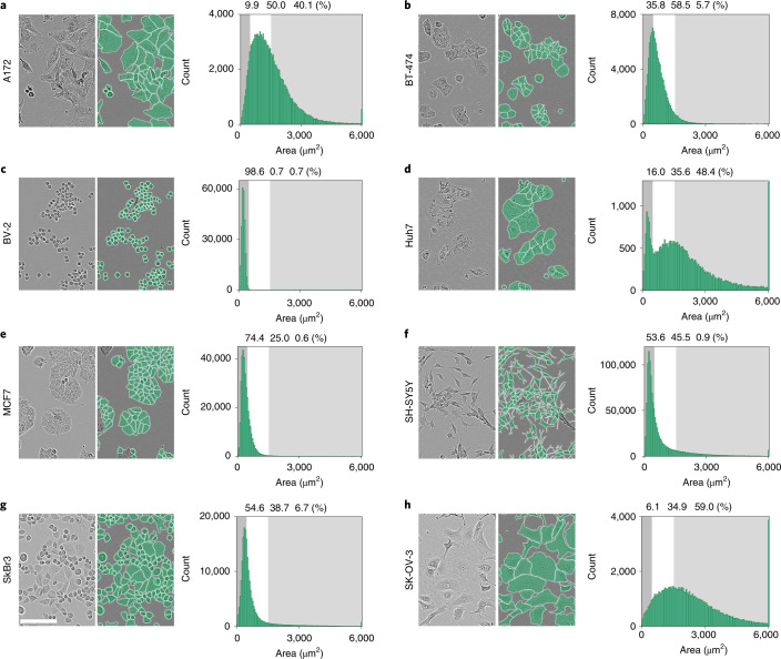
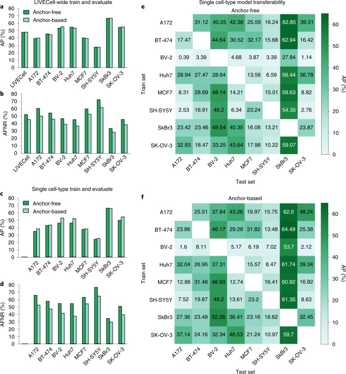
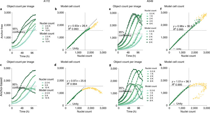
Light microscopy combined with well-established protocols of two-dimensional cell culture facilitates high-throughput quantitative imaging to study biological phenomena. Accurate segmentation of individual cells in images enables exploration of complex biological questions, but can require sophisticated imaging processing pipelines in cases of low contrast and high object density. Deep learning-based methods are considered state-of-the-art for image segmentation but typically require vast amounts of annotated data, for which there is no suitable resource available in the field of label-free cellular imaging. Here, we present LIVECell, a large, high-quality, manually annotated and expert-validated dataset of phase-contrast images, consisting of over 1.6 million cells from a diverse set of cell morphologies and culture densities. To further demonstrate its use, we train convolutional neural network-based models using LIVECell and evaluate model segmentation accuracy with a proposed a suite of benchmarks.
Overview
The claims and statistics of this paper haven’t been checked yet.
Run the check — free, no account needed. It reads the open-access text and checks the sources it cites.
Integrity signals
Registry
Cites
Statistics
Figures
Verification
Claims the paper makes
The claims and statistics of this paper haven’t been checked yet.
Run the check — free, no account needed. It reads the open-access text and checks the sources it cites.
Claims other papers make about this one
Each is checked against this paper’s own text: does it say what the citing paper says it does?
The source backs part of the claim, not all of it — or backs it for a different population, condition or comparison.
In the citing paper
“The LiveCell dataset consists of 3,188 training and 1,516 test images of eight different cell lines collected using phase-contrast microscopy, and each image has manual segmentations of the cells (https://sartorius-research.github.io/LIVECell/)7.”
From Cellpose 2.0: how to train your own model (2022) · cites this paper as [7]
Experimental — accuracy not yet measured
Self-check
Percentages, sums and reported differences re-computed from the paper’s own numbers.
The self-check needs the paper’s full text.
Citations
Cites
U-Net: Convolutional Networks for Biomedical Image Segmentation
Ronneberger, O., Fischer, P., & Brox, T. (2015) · Lecture notes in computer science · doi:10.1007/978-3-319-24574-4_28 · Cited by 99,404
An Image is Worth 16x16 Words: Transformers for Image Recognition at Scale
Dosovitskiy, A., Beyer, L., Kolesnikov, A., Weissenborn, D., Zhai, X., Unterthiner, T., Dehghani, M., Minderer, M., Heigold, G., Gelly, S., et al. (2020) · arXiv · doi:10.48550/arxiv.2010.11929 · Cited by 47,472
Microsoft COCO: Common Objects in Context
Lin, T.-Y., Maire, M., Belongie, S., Hays, J., Perona, P., Ramanan, D., Dollár, P., & Zitnick, C. L. (2014) · Lecture Notes in Computer Science · doi:10.1007/978-3-319-10602-1_48 · Cited by 45,460
PyTorch: An Imperative Style, High-Performance Deep Learning Library
Paszke, A., Gross, S., Massa, F., Lerer, A., Bradbury, J., Chanan, G., Killeen, T., Lin, Z., Gimelshein, N., Antiga, L., et al. (2019) · arXiv · doi:10.48550/arxiv.1912.01703 · Cited by 31,473
FCOS: Fully Convolutional One-Stage Object Detection
Tian, Z., Shen, C., Chen, H., & He, T. (2019) · 2019 IEEE/CVF International Conference on Computer Vision (ICCV) · doi:10.1109/iccv.2019.00972 · Cited by 7,013
CellProfiler: image analysis software for identifying and quantifying cell phenotypes
Carpenter, A. E., Jones, T. R., Lamprecht, M. R., Clarke, C., Kang, I. H., Friman, O., Guertin, D. A., Chang, J. H., Lindquist, R. A., Moffat, J., et al. (2006) · Genome biology · doi:10.1186/gb-2006-7-10-r100 · Cited by 5,212
Cellpose: a generalist algorithm for cellular segmentation
Stringer, C., Wang, T., Michaelos, M., & Pachitariu, M. (2021) · Nature Methods · doi:10.1038/s41592-020-01018-x · Cited by 4,369
Kuznetsova, A., Rom, H., Alldrin, N., Uijlings, J., Krasin, I., Pont-Tuset, J., Kamali, S., Popov, S., Malloci, M., Kolesnikov, A., et al. (2018) · arXiv (Cornell University) · doi:10.48550/arxiv.1811.00982 · Cited by 2,194
ResNeSt: Split-Attention Networks
Zhang, H., Wu, C., Zhang, Z., Zhu, Y., Lin, H., Zhang, Z., Sun, Y., He, T., Mueller, J. W., Manmatha, R., et al. (2022) · IEEE/CVF Conference on Computer Vision and Pattern Recognition Workshops (CVPRW) · doi:10.1109/cvprw56347.2022.00309 · Cited by 2,115
Cascade R-CNN: High Quality Object Detection and Instance Segmentation
Cai, Z., & Vasconcelos, N. M. (2019) · IEEE Transactions on Pattern Analysis and Machine Intelligence · doi:10.1109/tpami.2019.2956516 · Cited by 2,062
Research works printed but not linked: 1
- Levene, H. in Contributions to Probability and Statistics: Essays in Honor of Harold Hotelling (eds Olkin, I. et al.) 279–292 (Stanford Univ. Press, 1961).
Cited by
Sorted by citations
Cellpose 2.0: how to train your own model
Pachitariu, M., & Stringer, C. (2022) · Nature Methods · doi:10.1038/s41592-022-01663-4 · Cited by 1,381
Cellpose3: one-click image restoration for improved cellular segmentation
Stringer, C., & Pachitariu, M. (2025) · Nature Methods · doi:10.1038/s41592-025-02595-5 · Cited by 557
Segment Anything for Microscopy
Archit, A., Freckmann, L., Nair, S., Khalid, N., Hilt, P., Rajashekar, V., Freitag, M., Teuber, C., Spitzner, M., Contreras, C. T., et al. (2025) · Nature Methods · doi:10.1038/s41592-024-02580-4 · Cited by 426
Self-citationCellpose-SAM: superhuman generalization for cellular segmentationPreprint
Pachitariu, M., Rariden, M., & Stringer, C. (2025) · bioRxiv (Cold Spring Harbor Laboratory) · doi:10.1101/2025.04.28.651001 · Cited by 402
A guide to artificial intelligence for cancer researchers
Pérez-López, R., Laleh, N. G., Mahmood, F., & Kather, J. N. (2024) · Nature reviews. Cancer · doi:10.1038/s41568-024-00694-7 · Cited by 227
The multimodality cell segmentation challenge: toward universal solutions
Ma, J., Xie, R., Ayyadhury, S., Ge, C., Gupta, A., Gupta, R., Gu, S., Zhang, Y., Lee, G., Kim, J., et al. (2024) · Nature Methods · doi:10.1038/s41592-024-02233-6 · Cited by 154
Bridging live-cell imaging and next-generation cancer treatment
Alieva, M., Wezenaar, A. K. L., Wehrens, E. J., & Rios, A. C. (2023) · Nature reviews. Cancer · doi:10.1038/s41568-023-00610-5 · Cited by 84
Nuclei segmentation using attention aware and adversarial networks
Göçeri, E. (2024) · Neurocomputing · doi:10.1016/j.neucom.2024.127445 · Cited by 81
Nucleus segmentation: towards automated solutions
Hollandi, R., Moshkov, N., Paavolainen, L., Tasnádi, E., Piccinini, F., & Horváth, P. (2022) · Trends in Cell Biology · doi:10.1016/j.tcb.2021.12.004 · Cited by 82
Vanrobaeys, Y. S., Peterson, Z. J., Walsh, E. N., Chatterjee, S., Lin, L., Lyons, L. C., Nickl‐Jockschat, T., & Abel, T. G. (2023) · Nature Communications · doi:10.1038/s41467-023-42751-z · Cited by 75
CellSAM: A Foundation Model for Cell SegmentationPreprint
Israel, U., Marks, M., Dilip, R., Li, Q., Yu, C., Laubscher, E., Iqbal, A., Pradhan, E., Ates, A., Abt, M., et al. (2023) · bioRxiv (Cold Spring Harbor Laboratory) · doi:10.1101/2023.11.17.567630 · Cited by 64
Towards foundation models of biological image segmentation
Ma, J., & Wang, B. (2023) · Nature Methods · doi:10.1038/s41592-023-01885-0 · Cited by 57
Ultrack: pushing the limits of cell tracking across biological scales
Bragantini, J., Theodoro, I., Zhao, X., Huijben, T. A. P. M., Hirata-Miyasaki, E., VijayKumar, S., Balasubramanian, A., Lao, T., Agrawal, R., Xiao, S., et al. (2025) · Nature Methods · doi:10.1038/s41592-025-02778-0 · Cited by 63
Artificial intelligence for high content imaging in drug discovery
Puigvert, J. C., & Spjuth, O. (2024) · Current Opinion in Structural Biology · doi:10.1016/j.sbi.2024.102842 · Cited by 55
Segmentation metric misinterpretations in bioimage analysis
Hirling, D., Tasnádi, E., Caicedo, J. C., Caroprese, M., Sjögren, R., Aubreville, M., Koós, K., & Horváth, P. (2023) · Nature Methods · doi:10.1038/s41592-023-01942-8 · Cited by 46
Self-citationCellSAM: a foundation model for cell segmentation
Marks, M., Israel, U., Dilip, R., Li, Q., Yu, C., Laubscher, E., Iqbal, A., Pradhan, E., Ates, A., Abt, M., et al. (2025) · Nature Methods · doi:10.1038/s41592-025-02879-w · Cited by 152
Efficient end-to-end learning for cell segmentation with machine generated weak annotations
Shrestha, P., Kuang, N., & Yu, J. (2023) · Communications Biology · doi:10.1038/s42003-023-04608-5 · Cited by 50
Metlek, S. (2024) · Neural Computing and Applications · doi:10.1007/s00521-023-09374-3 · Cited by 44
Kaza, N., Ojaghi, A., & Robles, F. E. (2022) · BME Frontiers · doi:10.34133/2022/9853606 · Cited by 38
Practical guidelines for cell segmentation models under optical aberrations in microscopy
Peng, B., Chen, J., Githinji, P. B., Gul, I., Ye, Q., Chen, M., Qin, P., Huang, X., Yan, C. C., Yu, D., et al. (2024) · Computational and Structural Biotechnology Journal · doi:10.1016/j.csbj.2024.09.002 · Cited by 40
Induced Pluripotent Stem Cell-Based Drug Screening by Use of Artificial Intelligence
Kusumoto, D., Yuasa, S., & Fukuda, K. (2022) · Pharmaceuticals · doi:10.3390/ph15050562 · Cited by 37
OPLS-Based Multiclass Classification and Data-Driven Interclass Relationship Discovery
Forsgren, E., Björkblom, B., Trygg, J., & Jonsson, P. (2025) · Journal of Chemical Information and Modeling · doi:10.1021/acs.jcim.4c01799 · Cited by 36
Self-citationChen, K., Zhou, Y., Ding, M., Wang, Y., Ren, Z., & Yang, Y. (2023) · bioRxiv (Cold Spring Harbor Laboratory) · doi:10.1101/2023.01.31.526427 · Cited by 37
A systematic evaluation of computational methods for cell segmentation
Wang, Y., Zhao, J., Xu, H., Han, C., Tao, Z., Zhou, D., Geng, T., Liu, D., & Ji, Z. (2024) · Briefings in Bioinformatics · doi:10.1093/bib/bbae407 · Cited by 36
Schroeder, A. R., Loth, M., Luo, C., Yao, S., Yan, H., Zhang, D., Piya, S., Plowey, E. D., Hu, W., Clemenceau, J. R. V., et al. (2025) · Nature Methods · doi:10.1038/s41592-025-02770-8 · Cited by 37
Wünnemann, F., Sicklinger, F., Bestak, K., Nimo, J., Thiemann, T., Amrute, J., Nordbeck, M., Hartmann, N., Ibarra-Arellano, M. A., Tanevski, J., et al. (2025) · Nature Cardiovascular Research · doi:10.1038/s44161-025-00717-y · Cited by 37
Optofluidic imaging meets deep learning: from merging to emerging
Siu, D. M. D., Lee, K. C. M., Chung, B. M. F., Wong, J. S. J., Zheng, G., & Tsia, K. K. (2023) · Lab on a Chip · doi:10.1039/d2lc00813k · Cited by 30
Deep Learning in Single-cell Analysis
Molho, D., Ding, J., Tang, W., Li, Z., Wen, H., Wang, Y., Venegas, J., Jin, W., Liu, R., Su, R., et al. (2024) · ACM Transactions on Intelligent Systems and Technology · doi:10.1145/3641284 · Cited by 38
Label-free tumor cells classification using deep learning and high-content imaging
Piansaddhayanon, C., Koracharkornradt, C., Laosaengpha, N., Tao, Q., Ingrungruanglert, P., Israsena, N., Chuangsuwanich, E., & Sriswasdi, S. (2023) · Scientific Data · doi:10.1038/s41597-023-02482-8 · Cited by 28
Deep Learning in Cell Image Analysis
Xu, J., Zhou, D., Deng, D., Li, J., Chen, C., Liao, X., Chen, G., & Heng, P. (2022) · Intelligent Computing · doi:10.34133/2022/9861263 · Cited by 30
Zargari, A., Topacio, B. R., Mashhadi, N., & Shariati, S. A. (2024) · iScience · doi:10.1016/j.isci.2024.109740 · Cited by 26
Spatial single-cell omics: new insights into liver diseases
Suo, Y., Thimme, R., & Bengsch, B. (2025) · Gut · doi:10.1136/gutjnl-2024-332105 · Cited by 29
Self-supervised machine learning for live cell imagery segmentation
Robitaille, M. C., Byers, J. M., Christodoulides, J. A., & Raphael, M. P. (2022) · Communications Biology · doi:10.1038/s42003-022-04117-x · Cited by 31
Sockell, A., Wong, W. H., Longwell, S. A., Vu, T., Karlsson, K., Mokhtari, D. A., Schaepe, J. M., Lo, Y., Cornelius, V., Kuo, C. J., et al. (2023) · Cell Systems · doi:10.1016/j.cels.2023.08.002 · Cited by 25
Maddalena, L., Antonelli, L., Albu, A., Hada, A., & Guarracino, M. R. (2022) · Algorithms · doi:10.3390/a15090313 · Cited by 24
MIA is an open-source standalone deep learning application for microscopic image analysis
Körber, N. (2023) · Cell Reports Methods · doi:10.1016/j.crmeth.2023.100517 · Cited by 23
Mantis: High-throughput 4D imaging and analysis of the molecular and physical architecture of cells
Ivanov, I. E., Hirata-Miyasaki, E., Chandler, T., Cheloor-Kovilakam, R., Liu, Z., Pradeep, S., Liu, C., Bhave, M., Khadka, S., Arias, C., et al. (2024) · PNAS Nexus · doi:10.1093/pnasnexus/pgae323 · Cited by 21
Chen, B., Yin, Z., Ng, W., Wang, D. M., Tuan, R. S., Bise, R., & Ker, D. F. E. (2024) · npj Imaging · doi:10.1038/s44303-024-00046-y · Cited by 23
Automating Ground Truth Annotations for Gland Segmentation Through Immunohistochemistry
Kataria, T., Rajamani, S., Ayubi, A. B., Bronner, M. P., Jedrzkiewicz, J., Knudsen, B. S., & Elhabian, S. (2023) · Modern Pathology · doi:10.1016/j.modpat.2023.100331 · Cited by 21
Kim, M., & Hong, S. (2024) · Technologies · doi:10.3390/technologies12070095 · Cited by 28
Casti, P., Cardarelli, S., Comes, M. C., D’Orazio, M., Filippi, J., Antonelli, G., Mencattini, A., Natale, C. D., & Martinelli, E. (2023) · Expert Systems with Applications · doi:10.1016/j.eswa.2023.120861 · Cited by 19
SOAPy: a Python package to dissect spatial architecture, dynamics, and communication
Wang, H., Li, J., Jing, S., Lin, P., Qiu, Y., Yan, X., Yuan, J., Tang, Z., Li, Y., Zhang, H., et al. (2025) · Genome biology · doi:10.1186/s13059-025-03550-5 · Cited by 20
A survey of deep learning methods on cell instance segmentation
Wang, C., Lee, W.-T., & Su, T.-S. (2025) · Neural Computing and Applications · doi:10.1007/s00521-025-11119-3 · Cited by 21
Transforming microfluidics for single-cell analysis with robotics and artificial intelligence
Cheng, J., Anne, R., & Chen, Y. (2025) · Lab on a Chip · doi:10.1039/d5lc00216h · Cited by 21
Defining the boundaries: challenges and advances in identifying cells in microscopy images
Gogoberidze, N., & Cimini, B. A. (2023) · Current Opinion in Biotechnology · doi:10.1016/j.copbio.2023.103055 · Cited by 18
SortedAP: Rethinking evaluation metrics for instance segmentation
Chen, L., Wu, Y., Stegmaier, J., & Merhof, D. (2023) · IEEE International Conference on Computer Vision Workshops · doi:10.1109/iccvw60793.2023.00424 · Cited by 16
Daus, S., Buchwald, T., & Peuker, U. A. (2024) · Powder Technology · doi:10.1016/j.powtec.2024.119884 · Cited by 16
He, S., Sillah, M., Cole, A. R., Uboveja, A., Aird, K. M., Chen, Y., & Gong, Y. (2024) · Cells · doi:10.3390/cells13121004 · Cited by 16
Deep-Manager: a versatile tool for optimal feature selection in live-cell imaging analysis
Mencattini, A., D’Orazio, M., Casti, P., Comes, M. C., Giuseppe, D. D., Antonelli, G., Filippi, J., Corsi, F., Ghibelli, L., Veith, I., et al. (2023) · Communications Biology · doi:10.1038/s42003-023-04585-9 · Cited by 15
EPC-DARTS: Efficient partial channel connection for differentiable architecture search
Cai, Z., Chen, L., & Liu, H. (2023) · Neural Networks · doi:10.1016/j.neunet.2023.07.029 · Cited by 15
Pan, F., Wu, Y., Cui, K., Chen, S., Li, Y., Liu, Y., Shakoor, A., Zhao, H., Lu, B., Zhi, S., et al. (2024) · Computers in Biology and Medicine · doi:10.1016/j.compbiomed.2024.109151 · Cited by 15
Naumenko, E., Guryanov, I., Zakirova, E. Y., & Fakhrullin, R. F. (2021) · Polymers · doi:10.3390/polym13223949 · Cited by 15
Machine learning-based detection of label-free cancer stem-like cell fate
Chambost, A. J., Berabez, N., Cochet‐Escartin, O., Ducray, F., Gabut, M., Isaac, C., Martel, S., Idbaïh, A., Rousseau, D., Meyronet, D., et al. (2022) · Scientific Reports · doi:10.1038/s41598-022-21822-z · Cited by 16
Robust virtual staining of landmark organelles with Cytoland
Liu, Z., Hirata-Miyasaki, E., Pradeep, S., Rahm, J. V., Foley, C., Chandler, T., Ivanov, I. E., Woosley, H. O., Lee, S.-C., Khadka, S., et al. (2025) · Nature Machine Intelligence · doi:10.1038/s42256-025-01046-2 · Cited by 25
Gu, Z., Wang, S., Rong, R., Zhao, Z., Wu, F., Zhou, Q., Wen, Z., Chi, Z., Fang, Y. V., Peng, Y., et al. (2024) · Laboratory Investigation · doi:10.1016/j.labinv.2024.102184 · Cited by 16
Cellular analysis using label-free parallel array microscopy with Fourier ptychography
Wakefield, D. L., Graham, R., Wong, K., Wang, S., Hale, C. M., & Yu, C. (2022) · Biomedical Optics Express · doi:10.1364/boe.451128 · Cited by 15
Liu, J., Jiang, Z., Cao, T., Chen, Z., Zhang, C., & Gui, W. (2022) · IEEE Transactions on Circuits and Systems for Video Technology · doi:10.1109/tcsvt.2022.3230451 · Cited by 13
Transformer-based Detection of Microorganisms on High-Resolution Petri Dish Images
Ebert, N., Stricker, D., & Wasenmüller, O. (2023) · IEEE International Conference on Computer Vision Workshops · doi:10.1109/iccvw60793.2023.00428 · Cited by 13
A novel deep learning graph attention network for Alzheimer’s disease image segmentation
Hasan, E., & Wagler, A. E. (2024) · Healthcare Analytics · doi:10.1016/j.health.2024.100310 · Cited by 13
Hou, W., Liu, Q., Ma, H., Qu, Y., & Ji, Z. (2025) · Advanced Intelligent Systems · doi:10.1002/aisy.202400947 · Cited by 13
Point2Mask: A Weakly Supervised Approach for Cell Segmentation Using Point Annotation
Khalid, N., Schmeisser, F., Koochali, M., Munir, M., Edlund, C., Jackson, T. R., Trygg, J., Sjögren, R., Dengel, A. R., & Ahmed, S. (2022) · Lecture notes in computer science · doi:10.1007/978-3-031-12053-4_11 · Cited by 13
Self-citationMicrosnoop: A generalist tool for microscopy image representation
Xun, D., Wang, R., Zhang, X., & Wáng, Y. (2024) · The Innovation · doi:10.1016/j.xinn.2023.100541 · Cited by 14
Trizna, E. Y., Sinitca, A., Lyanova, A. I., Baidamshina, D. R., Zelenikhin, P., Kaplun, D., Kayumov, A. R., & Bogachev, M. I. (2023) · Scientific Data · doi:10.1038/s41597-023-02065-7 · Cited by 15
A self-supervised learning approach for high throughput and high content cell segmentation
Lam, V. K., Byers, J. M., Robitaille, M. C., Kaler, L., Christodoulides, J. A., & Raphael, M. P. (2025) · Communications Biology · doi:10.1038/s42003-025-08190-w · Cited by 18
Zhou, Y., Li, W., & Yang, G. (2023) · IEEE Winter Conference on Applications of Computer Vision · doi:10.1109/wacv56688.2023.00589 · Cited by 12
CellT-Net: A Composite Transformer Method for 2-D Cell Instance Segmentation
Wan, Z., Li, M., Wang, Z., Tan, H., Li, W., Yu, L., & Samuel, R. D. J. (2023) · IEEE Journal of Biomedical and Health Informatics · doi:10.1109/jbhi.2023.3265006 · Cited by 12
Wang, J., Zhang, Z., Wu, M., Ye, Y., Wang, S., Cao, Y., & Yang, H. (2023) · Computers in Biology and Medicine · doi:10.1016/j.compbiomed.2023.107622 · Cited by 12
Marx, D. H., Kumar, K., & Zornberg, J. G. (2023) · Geotextiles and Geomembranes · doi:10.1016/j.geotexmem.2023.04.004 · Cited by 14
PACE: Point Annotation-Based Cell Segmentation for Efficient Microscopic Image Analysis
Khalid, N., Fróes, T. C., Caroprese, M., Lovell, G. F., Trygg, J., Dengel, A., & Ahmed, S. (2023) · Lecture notes in computer science · doi:10.1007/978-3-031-44210-0_44 · Cited by 11
Self-citationВитальевич, С. М., Сергеевна, Ч. Е., Станиславовна, К. А., Akopyan, G. V., Turchyn, V. V., Геннадиевич, П. А., Filimonov, D., & Ishchenko, R. V. (2025) · International Journal of Molecular Sciences · doi:10.3390/ijms26052338 · Cited by 11
Xun, D., Chen, D., Zhou, Y., Lauschke, V. M., Wang, R., & Wáng, Y. (2022) · iScience · doi:10.1016/j.isci.2022.105506 · Cited by 13
Exploring the Impact of Variability in Cell Segmentation and Tracking Approaches
Wiggins, L., O’Toole, P. J., Brackenbury, W. J., & Wilson, J. C. (2024) · Microscopy Research and Technique · doi:10.1002/jemt.24715 · Cited by 14
Wang, C., Wan, Y., Li, S., Qu, K., Zhou, X., He, J., Ke, J., Yu, Y., Wang, T., & Shen, Y. (2024) · IEEE Transactions on Medical Imaging · doi:10.1109/tmi.2024.3501352 · Cited by 13
SAMCell: Generalized label-free biological cell segmentation with segment anything
VandeLoo, A. D., Malta, N. J., Sanganeriya, S., Aponte, E., van Zyl, C., Xu, D., & Forest, C. R. (2025) · PLoS ONE · doi:10.1371/journal.pone.0319532 · Cited by 10
DeepMuCS: A Framework for Co-culture Microscopic Image Analysis: From Generation to Segmentation
Khalid, N., Koochali, M., Rajashekar, V., Munir, M., Edlund, C., Jackson, T. R., Trygg, J., Sjögren, R., Dengel, A. R., & Ahmed, S. (2022) · IEEE-EMBS International Conference on Biomedical and Health Informatics (BHI ...) · doi:10.1109/bhi56158.2022.9926936 · Cited by 10
Self-citationMeierrieks, F., Kour, A., Pätz, M., Pflanz, K. B., Wolff, M. W., & Pickl, A. (2023) · Molecular Therapy — Methods & Clinical Development · doi:10.1016/j.omtm.2023.101118 · Cited by 10
Generalizable morphological profiling of cells by interpretable unsupervised learning
Murthy, R. S., Stassen, S. V., Siu, D. M. D., Lo, M. C. K., Yip, G. G. K., & Tsia, K. K. (2025) · Nature Communications · doi:10.1038/s41467-025-66267-w · Cited by 9
Automatic enhancement preprocessing for segmentation of low quality cell images
Kato, S., & Hotta, K. (2024) · Scientific Reports · doi:10.1038/s41598-024-53411-7 · Cited by 9
MMV_Im2Im: an open-source microscopy machine vision toolbox for image-to-image transformation
Sonneck, J., Zhou, Y., & Chen, J. (2024) · GigaScience · doi:10.1093/gigascience/giad120 · Cited by 7
A review of adaptable conventional image processing pipelines and deep learning on limited datasets
Münke, F. R., Schuetzke, J., Berens, F., & Reischl, M. (2024) · Machine Vision and Applications · doi:10.1007/s00138-023-01501-3 · Cited by 11
Super resolution-based methodology for self-supervised segmentation of microscopy images
Bommanapally, V., Abeyrathna, D. L. B., Chundi, P., & Subramaniam, M. (2024) · Frontiers in Microbiology · doi:10.3389/fmicb.2024.1255850 · Cited by 8
Yakovlev, E. V., Simkin, I. V., Shirokova, A. A., Kolotyeva, N. A., Novikova, S. V., Nasyrov, A. D., Denisenko, I. R., Gursky, K. D., Shishkov, I. N., Narzaeva, D. E., et al. (2024) · Scientific Reports · doi:10.1038/s41598-024-59773-2 · Cited by 8
Du, R. F., Carbonell, E. L., Huang, J., Liu, S., Wang, X., Shen, D. G., & Ke, J. (2025) · IEEE Transactions on Medical Imaging · doi:10.1109/tmi.2025.3551913 · Cited by 10
Tsiporenko, I., Chizhov, P., & Fishman, D. (2025) · Lecture notes in computer science · doi:10.1007/978-3-031-91721-9_14 · Cited by 8
Zulueta-Coarasa, T., Jug, F., Mathur, A., Moore, J., Muñoz‐Barrutia, A., Anita, L., Babalola, K., Bankhead, P., Paul‐Gilloteaux, P., Gogoberidze, N., et al. (2025) · Nature Methods · doi:10.1038/s41592-025-02835-8 · Cited by 14
Dasdemir, E., Veletić, I., Ly, C. P., Quesada, A. E., Pacheco, C. D., Jelloul, F. Z., Borges, P., Basu, S., Jindal, S., Wang, Z., et al. (2025) · iScience · doi:10.1016/j.isci.2025.114289 · Cited by 9
Progress and new challenges in image-based profiling
Serrano, E., Peters, J., Wagner, J., Graham, R. E., Chen, Z., Feng, B. Y., Miranda, G., Kalinin, A. A., Vulliard, L., Tomkinson, J., et al. (2026) · Molecular Systems Biology · doi:10.1038/s44320-026-00197-7 · Cited by 18
Temporal and Locational Values of Images Affecting the Deep Learning of Cancer Stem Cell Morphology
Hanai, Y., Ishihata, H., Zhang, Z., Maruyama, R., Kasai, T., Kameda, H., & Sugiyama, T. (2022) · Biomedicines · doi:10.3390/biomedicines10050941 · Cited by 8
Label-free microscopy for virus infections
Petkidis, A., Andriasyan, V., & Greber, U. F. (2023) · Microscopy · doi:10.1093/jmicro/dfad024 · Cited by 8
Point-Supervised Single-Cell Segmentation via Collaborative Knowledge Sharing
Yu, J. H. (2023) · IEEE Transactions on Medical Imaging · doi:10.1109/tmi.2023.3312988 · Cited by 10
Brun, A., Mougeot, G., Denis, P., Collin, M., Pouchin, P., Montaurier, C., Walrand, S., Capel, F., & Gueugneau, M. (2024) · Scientific Reports · doi:10.1038/s41598-024-53658-0 · Cited by 8
A Comparative Analysis of Filter and Optimization Methods for Feature Selection
Reddy, K. G., Basha, M. M., & Mishra, D. (2023) · International Conference on Innovative Computing, Intelligent Communication and Smart Electrical Systems (ICSES) · doi:10.1109/icses60034.2023.10465517 · Cited by 8
MaxSigNet: Light learnable layer for semantic cell segmentation
Yazdi, R., & Khotanlou, H. (2024) · Biomedical Signal Processing and Control · doi:10.1016/j.bspc.2024.106464 · Cited by 8
Corallo, D., Vecchia, M. D., Lazic, D., Taschner‐Mandl, S., Biffi, A., & Aveic, S. (2023) · Biochemical Pharmacology · doi:10.1016/j.bcp.2023.115696 · Cited by 9
Antonelli, L., Polverino, F., Albu, A., Hada, A., Asteriti, I. A., Degrassi, F., Guarguaglini, G., Maddalena, L., & Guarracino, M. R. (2023) · Scientific Data · doi:10.1038/s41597-023-02540-1 · Cited by 8
Zhong, L., Li, L., & Yang, G. (2024) · BMC Bioinformatics · doi:10.1186/s12859-024-05894-4 · Cited by 7
A Survey of Deep Learning in Histopathological Nuclear Segmentation
Qin, L., Yang, X., Xu, X., & Zhu, Z. (2025) · IEEE Computational Intelligence Magazine · doi:10.1109/mci.2025.3564274 · Cited by 7
From images to understanding: Advances in deep learning for cellular dynamics analysis
Woodhams, B., & Uhlmann, V. (2025) · Current Opinion in Cell Biology · doi:10.1016/j.ceb.2025.102585 · Cited by 6
Pizzagalli, D. U., Carrillo-Barberà, P., Bansal, H., Palladino, E., Ceni, K., Thelen, B., Pulfer, A., Moscatello, E., Cabini, R. F., Textor, J. C., et al. (2025) · The EMBO Journal · doi:10.1038/s44318-025-00629-4 · Cited by 7
A nasal cytology dataset for object detection and deep learning
Camporeale, M. G., Dimauro, G., Gelardi, M., Iacobellis, G., Ladisa, M. S., Latrofa, S., & Lomonte, N. (2025) · Biomedical Signal Processing and Control · doi:10.1016/j.bspc.2025.109263 · Cited by 7
Metadata
- Authors
- Edlund, C., Jackson, T. R., Khalid, N., Bevan, N., Dale, T., Dengel, A., Ahmed, S., Trygg, J., & Sjögren, R.
- Affiliations
- Sartorius (United Kingdom) (GB)
- German Research Centre for Artificial Intelligence (DE)
- Umeå University (SE)
- Corresponding author
- Sjögren, Rickard
- ORCID
- Venue
- Nature Methods
- Published
- 2021-08-30
- Volume
- 18
- Issue
- 9
- Pages
- 1038-1045
- ISSN
- 1548-7091 (ISSN-L)
- 1548-7105
- PMC
- PMC8440198
- OpenAlex
- W3196890347
- Cited by
- 304
- References
- 29
- Citations by year
- 2026: 56 · 2025: 88 · 2024: 63 · 2023: 65 · 2022: 31 · 2021: 1
- FWCI
- 18.09
- Type
- journal article
- Language
- en
- Open access
- hybrid
- doi.org
- Locations
- Nature Methods (publishedVersion, cc-by)
- Europe PMC (PubMed Central) (publishedVersion, other-oa)
- PubMed Central (publishedVersion, cc-by)
- PubMed (publishedVersion)
- DiVA at Umeå University (Umeå University) (submittedVersion, other-oa)
- Topics
- Life Sciences › Biochemistry, Genetics and Molecular Biology › Biophysics › Cell Image Analysis Techniques
- Physical Sciences › Computer Science › Computer Vision and Pattern Recognition › Advanced Neural Network Applications
- Physical Sciences › Computer Science › Computer Vision and Pattern Recognition › Medical Image Segmentation Techniques
- Keywords
- cell segmentation, label-free imaging, phase contrast microscopy, convolutional neural networks, segmentation benchmark, cell culture, high-throughput imaging, cell morphology
- MeSH terms
- Humans, Image Processing, Computer-Assisted, Microscopy, Models, Biological, Databases, Factual, Neural Networks, Computer, Cell Culture Techniques
About these checks
Registry, retraction, Cites and statistics results are computed, not judged, with one exception: a printed reference that no index lists is read once by a model before it counts as a citation error. Claims are extracted by a model and kept only when their quote appears verbatim in the text; each cited source is then checked, with a model’s help, for whether it says what the claim relies on. Those verdicts can be wrong — read the claim’s quote and the cited source before relying on one.
Statistics and arithmetic are recomputed, not judged.
Confidence bands are shown only for fields calibrated on our annotated test set. None is calibrated yet, so no band is shown.
What counts as a claim ›How we measure confidence ›How we check this ›
Are you an author, or do you see a problem with this page? Request a review
