

The DOI matches its Crossref record; 49 of the 54 references it cites were found in a registry or an index; none of the 25 sources its claims cite is checked for support yet.
Foundation model for cancer imaging biomarkers
Open accessAbstract
Foundation models in deep learning are characterized by a single large-scale model trained on vast amounts of data serving as the foundation for various downstream tasks. Foundation models are generally trained using self-supervised learning and excel in reducing the demand for training samples in downstream applications. This is especially important in medicine, where large labelled datasets are often scarce. Here, we developed a foundation model for cancer imaging biomarker discovery by training a convolutional encoder through self-supervised learning using a comprehensive dataset of 11,467 radiographic lesions. The foundation model was evaluated in distinct and clinically relevant applications of cancer imaging-based biomarkers. We found that it facilitated better and more efficient learning of imaging biomarkers and yielded task-specific models that significantly outperformed conventional supervised and other state-of-the-art pretrained implementations on downstream tasks, especially when training dataset sizes were very limited. Furthermore, the foundation model was more stable to input variations and showed strong associations with underlying biology. Our results demonstrate the tremendous potential of foundation models in discovering new imaging biomarkers that may extend to other clinical use cases and can accelerate the widespread translation of imaging biomarkers into clinical settings.
Overview
AI snapshot
Written from the paper’s full text.
TL;DR
A 3D ResNet50 foundation model was pretrained with a modified SimCLR objective on 11,467 CT lesions from 2,312 patients and evaluated on anatomical site classification, lung nodule malignancy, and NSCLC prognosis. It improved downstream imaging-biomarker performance, especially with limited training data, and showed stability and biological associations.
Key findings
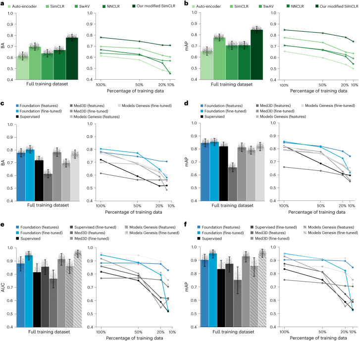
- Modified SimCLR pretraining outperformed auto-encoder, SimCLR, SwAV, and NNCLR on lesion anatomical site classification, achieving balanced accuracy 0.779 (95% CI 0.750–0.810) and mAP 0.847 (95% CI 0.750–0.810); SimCLR was second best with balanced accuracy 0.696 (95% CI 0.663–0.728) and mAP 0.779 (95% CI 0.749–0.811).
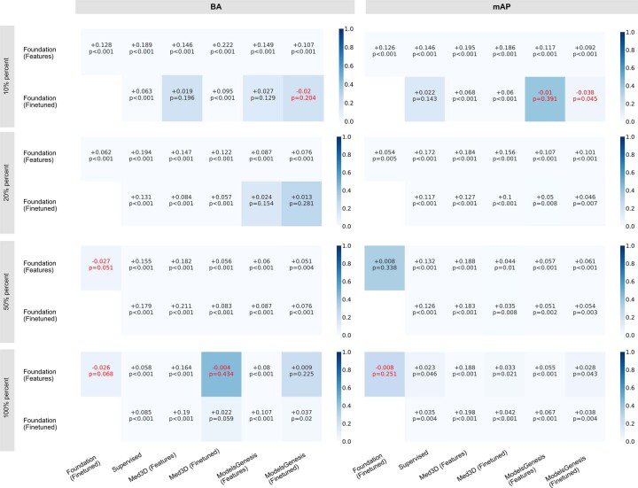
- For lesion anatomical site classification (use case 1), Foundation (fine-tuned) reached mAP 0.857 (95% CI 0.828–0.886) and balanced accuracy 0.804 (95% CI 0.775–0.835), significantly outperforming baselines on mAP and most baselines on balanced accuracy; Foundation (features) was especially robust under reduced training data.
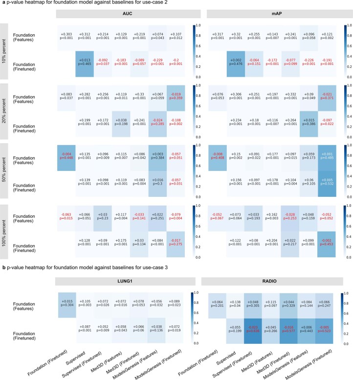
- For lung nodule malignancy (use case 2), Foundation (fine-tuned) achieved AUC 0.944 (95% CI 0.907–0.972) and mAP 0.953 (95% CI 0.915–0.979); Foundation (features) dominated baselines at 50%, 20%, and 10% training data (n = 254, 101, and 51).
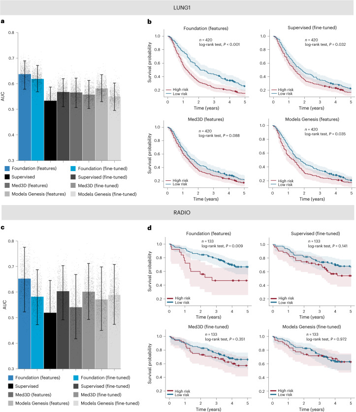
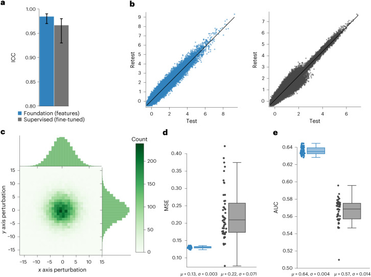
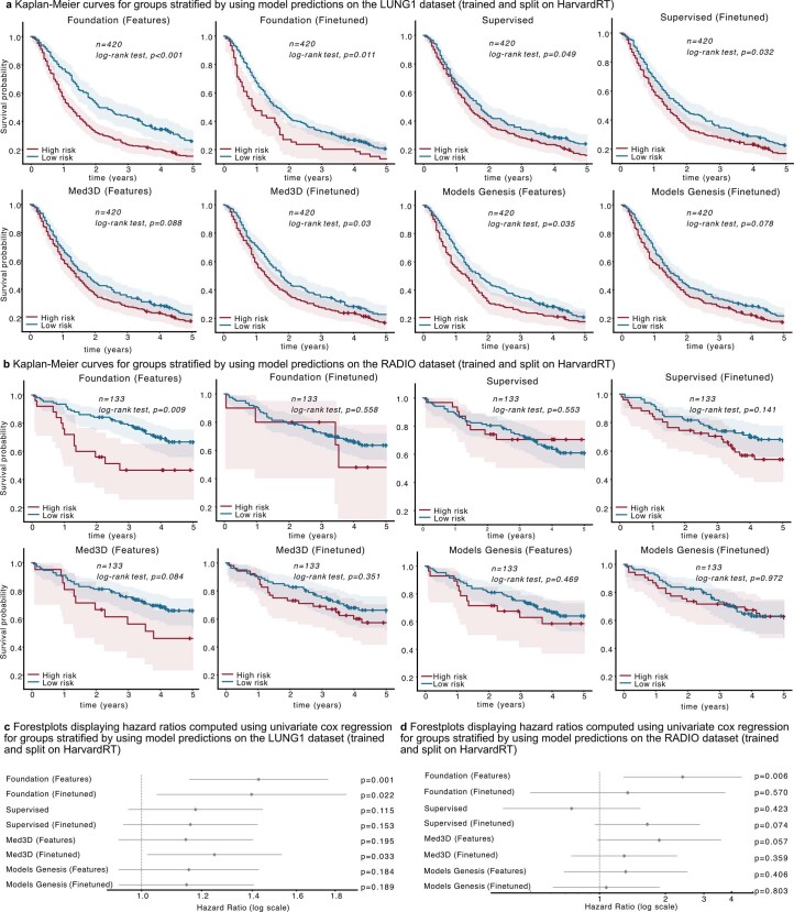
- For NSCLC prognostication (use case 3), Foundation (features) achieved AUC 0.638 (95% CI 0.584–0.692) on LUNG1 and AUC 0.653 (95% CI 0.532–0.771) on RADIO; it was the only model with significant Kaplan–Meier stratification on RADIO (P = 0.009), had test–retest ICC 0.984 versus 0.966 for Supervised (fine-tuned), and showed significantly higher absolute gene-expression correlations (P = 0.008) with immune-associated pathway enrichment.
Methods
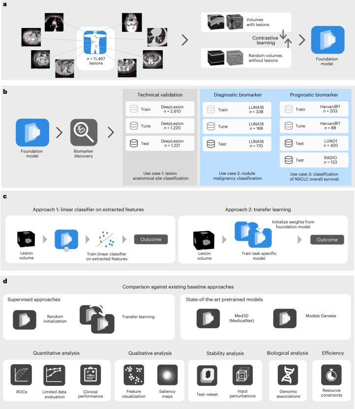
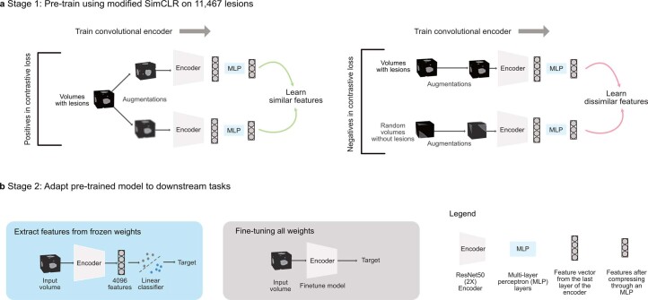
- Design: self-supervised contrastive pretraining of a 3D ResNet50 encoder using a modified SimCLR framework on 11,467 unlabelled CT lesions from 5,513 scans across 2,312 patients; downstream tasks used either frozen features with a logistic regression classifier or full fine-tuning.
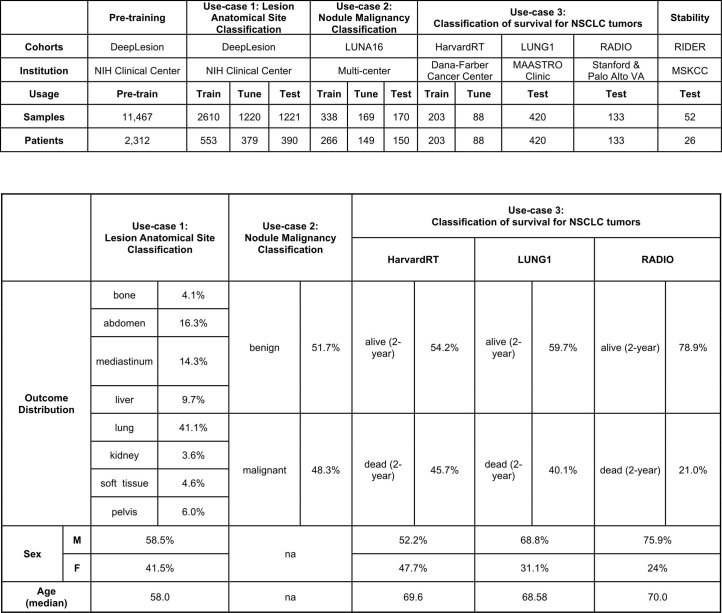
- Data: five datasets—DeepLesion, LUNA16, HarvardRT, LUNG1, and RADIO—covering three use cases: anatomical site classification (3,830 train/tune lesions; 1,221 test), nodule malignancy (338 train, 169 tune, 170 test nodules), and NSCLC 2-year overall survival (HarvardRT n = 291 train/tune; LUNG1 n = 420 and RADIO n = 133 test).
- Analysis: balanced accuracy and mAP for anatomical site, AUC-ROC for malignancy and prognosis, permutation tests with 1,000 permutations, bootstrap 95% CIs with 1,000 resamples, Kaplan–Meier/log-rank tests, stability analyses (ICC, MSE, perturbation trials), saliency maps, and gene-expression correlation plus gene-set enrichment analysis.
Limitations
- Stated by the paper: the study is retrospective; reliability across diverse demographic groups, distribution shifts, and biomarker tasks remains to be evaluated; larger pretraining data and integration of clinical covariates may be needed; deep-learning models remain “black box,” and saliency attribution methods have technical limitations; the biological association analysis is preliminary.
- Evident from the text: Models Genesis was excluded from use case 2 because it was pretrained on the same LUNA16 split, making comparison unfair due to overfitting; RADIO had a small sample size, so most model differences were not significant; reduced-training-data experiments were not performed for use case 3 because that use case already has inherently small sample sizes.
Model-written summary. Check it against the paper before relying on it.
Integrity signals
Registry
Cites
Statistics
Figures
Verification
Claims the paper makes
50 Own result · 16 Not checked yet · 16 Own interpretation · 6 No basis given · 4 Own method
A result the paper reports from its own data — it cites no other source for it, so there is none to check. The quote shows it is in the paper.
In the paper
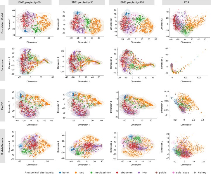
“We observed that features from the pretrained foundation model provided consistently interpretable and well-separated clusters across different settings.”
§ Foundation model for cancer imaging biomarkers > Results > Lesion anatomical site classification (use case 1)
plain- Asserted: passes — The authors put it forward as true.
- Checkable: passes — It can be checked against evidence.
- Load-bearing: passes — The paper’s conclusions depend on it.
- Based: passes — The paper gives a reason why it holds.
- Rests on an assumption: Access to large amounts of annotated data for specialized applications is often challenging and demands expertise, time and labour.
- Rests on an assumption: The quantity and quality of annotated data are strongly linked to the robustness of deep-learning models.
A result the paper reports from its own data — it cites no other source for it, so there is none to check. The quote shows it is in the paper.
In the paper
“Notably, none of the deep-learning fine-tuned baselines significantly improve over linear classification.”
§ Foundation model for cancer imaging biomarkers > Results > Nodule malignancy prediction (use case 2)
plain- Asserted: passes — The authors put it forward as true.
- Checkable: passes — It can be checked against evidence.
- Load-bearing: unclear — It is unclear whether the paper’s conclusions depend on it.
- Based: passes — The paper gives a reason why it holds.
- Rests on an assumption: Access to large amounts of annotated data for specialized applications is often challenging and demands expertise, time and labour.
- Rests on an assumption: The quantity and quality of annotated data are strongly linked to the robustness of deep-learning models.
A result the paper reports from its own data — it cites no other source for it, so there is none to check. The quote shows it is in the paper.
In the paper
“Moreover, when considering only mAP, the simple linear classification significantly (P < 0.05) outperformed all other implementations.”
§ Foundation model for cancer imaging biomarkers > Results > Lesion anatomical site classification (use case 1)
plaindirect- Asserted: passes — The authors put it forward as true.
- Checkable: passes — It can be checked against evidence.
- Load-bearing: passes — The paper’s conclusions depend on it.
- Based: passes — The paper gives a reason why it holds.
- Rests on an assumption: Access to large amounts of annotated data for specialized applications is often challenging and demands expertise, time and labour.
- Rests on an assumption: The quantity and quality of annotated data are strongly linked to the robustness of deep-learning models.
A result the paper reports from its own data — it cites no other source for it, so there is none to check. The quote shows it is in the paper.
In the paper
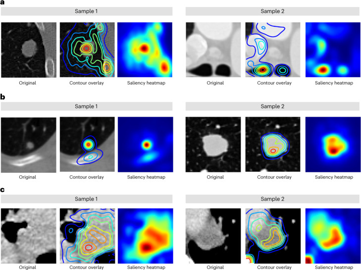
“Specifically, in use case 1 (Fig. 5a), the focus was mainly on areas surrounding the lesions, such as the parenchyma and bone regions in the lung and the trachea in mediastinal lesions.”
§ Foundation model for cancer imaging biomarkers > Results > Saliency maps for fine-tuned foundation models
plain- Asserted: passes — The authors put it forward as true.
- Checkable: passes — It can be checked against evidence.
- Load-bearing: unclear — It is unclear whether the paper’s conclusions depend on it.
- Based: passes — The paper gives a reason why it holds.
A result the paper reports from its own data — it cites no other source for it, so there is none to check. The quote shows it is in the paper.
In the paper
“Similar to the LUNG1 cohort, deep-learning implementations did not demonstrate superior performance (Fig. 3c).”
§ Foundation model for cancer imaging biomarkers > Results > NSCLC prognostication (use case 3)
plain- Asserted: passes — The authors put it forward as true.
- Checkable: passes — It can be checked against evidence.
- Load-bearing: passes — The paper’s conclusions depend on it.
- Based: passes — The paper gives a reason why it holds.
- Rests on an assumption: Access to large amounts of annotated data for specialized applications is often challenging and demands expertise, time and labour.
- Rests on an assumption: The quantity and quality of annotated data are strongly linked to the robustness of deep-learning models.
- Rests on an assumption: Image-biomarker studies for predicting endpoints such as overall survival on small cohorts largely rely on statistical feature extraction (engineered radiomics) and classical machine learning-based modelling.
- Rests on an assumption: These statistical feature extraction approaches require precise 3D segmentations, increasing the annotation burden of these studies.
A result the paper reports from its own data — it cites no other source for it, so there is none to check. The quote shows it is in the paper.
In the paper
“The auto-encoder approach, previously popular for pretraining, performed the worst compared to state-of-the-art contrastive SSL approaches.”
§ Foundation model for cancer imaging biomarkers > Results > Pretraining strategy selection
plain- Asserted: passes — The authors put it forward as true.
- Checkable: passes — It can be checked against evidence.
- Load-bearing: passes — The paper’s conclusions depend on it.
- Based: passes — The paper gives a reason why it holds.
- Rests on an assumption: Following pretraining, foundation models can be applied to task-specific problems, improving generalization, especially in tasks with small datasets.
A result the paper reports from its own data — it cites no other source for it, so there is none to check. The quote shows it is in the paper.
In the paper
“Regarding interpretability, we observed that models focused on varying regions of the tumour and surrounding tissue relevant to the associated use case.”
§ Foundation model for cancer imaging biomarkers > Discussion
plain- Asserted: passes — The authors put it forward as true.
- Checkable: passes — It can be checked against evidence.
- Load-bearing: unclear — It is unclear whether the paper’s conclusions depend on it.
- Based: passes — The paper gives a reason why it holds.
A result the paper reports from its own data — it cites no other source for it, so there is none to check. The quote shows it is in the paper.
In the paper
“Our analysis revealed that for each use case, the focus was primarily around tissues within or in proximity to the tumour”
§ Foundation model for cancer imaging biomarkers > Results > Saliency maps for fine-tuned foundation models
plain- Asserted: passes — The authors put it forward as true.
- Checkable: passes — It can be checked against evidence.
- Load-bearing: passes — The paper’s conclusions depend on it.
- Based: passes — The paper gives a reason why it holds.
None of the sources cited for this claim have been checked yet.
In the paper
“Features extracted from the foundation model, Foundation (features), when linearly classified, showed significantly improved performance in balanced accuracy and mAP over features extracted from Med3D (ref. 17) and Models Genesis18 baseline methods.”
§ Foundation model for cancer imaging biomarkers > Results > Lesion anatomical site classification (use case 1)
What the sources say
- Not checked yetcites [17] Chen, S., Ma, K. & Zheng, Y. Med3D: transfer learning for 3D medical image analysis. Preprint at https://arxiv.org/abs/1904.00625 (2019).
- Not checked yetcites [18] Zhou, Z. et al. Models Genesis: generic autodidactic models for 3D medical image analysis. Med. Image Comput. Comput. Assist. Interv. 11767, 384–393 (2019).
plaindirect- Asserted: passes — The authors put it forward as true.
- Checkable: passes — It can be checked against evidence.
- Load-bearing: passes — The paper’s conclusions depend on it.
- Based: passes — The paper gives a reason why it holds.
- Rests on an assumption: Access to large amounts of annotated data for specialized applications is often challenging and demands expertise, time and labour.
- Rests on an assumption: The quantity and quality of annotated data are strongly linked to the robustness of deep-learning models.
A result the paper reports from its own data — it cites no other source for it, so there is none to check. The quote shows it is in the paper.
In the paper
“Additionally, features and predictions from the foundation model features were found to be highly stable against inter-reader and test–retest variations.”
§ Foundation model for cancer imaging biomarkers > Discussion
plain- Asserted: passes — The authors put it forward as true.
- Checkable: passes — It can be checked against evidence.
- Load-bearing: passes — The paper’s conclusions depend on it.
- Based: passes — The paper gives a reason why it holds.
- It may state two separate claims as one. 25
- Probably not a substantial claim. 18
- The quote only partly states this claim. 2
A result the paper reports from its own data — it cites no other source for it, so there is none to check. The quote shows it is in the paper.
In the paper
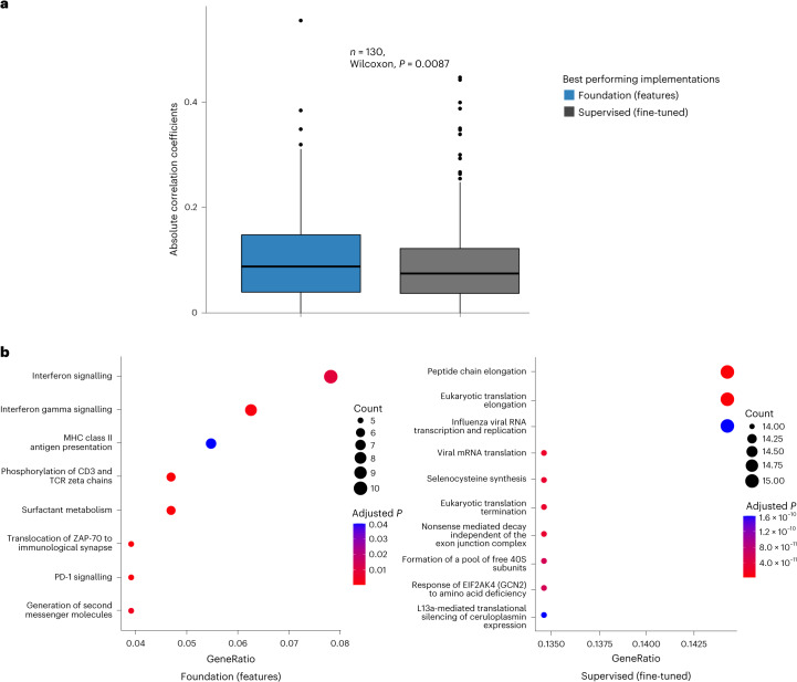
“Conversely, while the supervised model did show enrichment of individual pathways, no identifiable pattern was observed (Fig. 6b).”
§ Foundation model for cancer imaging biomarkers > Results > Underlying biological basis of the foundation model
plain- Asserted: passes — The authors put it forward as true.
- Checkable: passes — It can be checked against evidence.
- Load-bearing: unclear — It is unclear whether the paper’s conclusions depend on it.
- Based: passes — The paper gives a reason why it holds.
It may state two separate claims as one.
A result the paper reports from its own data — it cites no other source for it, so there is none to check. The quote shows it is in the paper.
In the paper
“Use case 3 (Fig. 5c) primarily attributed areas surrounding the centre of mass of the tumour, with some contribution from high-density bone regions.”
§ Foundation model for cancer imaging biomarkers > Results > Saliency maps for fine-tuned foundation models
plaincorrelational- Asserted: passes — The authors put it forward as true.
- Checkable: passes — It can be checked against evidence.
- Load-bearing: unclear — It is unclear whether the paper’s conclusions depend on it.
- Based: passes — The paper gives a reason why it holds.
It may state two separate claims as one.
A result the paper reports from its own data — it cites no other source for it, so there is none to check. The quote shows it is in the paper.
In the paper
“The implementation Med3D (fine-tuned), with AUC = 0.917 (95% CI 0.871–0.957) and mAP = 0.9307 (95% CI 0.888–0.964), performs slightly worse than our model, but this is not significant (P = 0.134).”
§ Foundation model for cancer imaging biomarkers > Results > Nodule malignancy prediction (use case 2)
plain- Asserted: passes — The authors put it forward as true.
- Checkable: passes — It can be checked against evidence.
- Load-bearing: passes — The paper’s conclusions depend on it.
- Based: passes — The paper gives a reason why it holds.
It may state two separate claims as one.
- Rests on an assumption: Access to large amounts of annotated data for specialized applications is often challenging and demands expertise, time and labour.
- Rests on an assumption: The quantity and quality of annotated data are strongly linked to the robustness of deep-learning models.
A result the paper reports from its own data — it cites no other source for it, so there is none to check. The quote shows it is in the paper.
In the paper
“Using these features provided the best performance on small cohorts in predicting prognosis and also demonstrated significant stratification of patients by their associated risk for each of the LUNG1 and RADIO cohorts (P < 0.01).”
§ Foundation model for cancer imaging biomarkers > Discussion
boostedcorrelational- Asserted: passes — The authors put it forward as true.
- Checkable: passes — It can be checked against evidence.
- Load-bearing: passes — The paper’s conclusions depend on it.
- Based: passes — The paper gives a reason why it holds.
It may state two separate claims as one.
- Rests on an assumption: Access to large amounts of annotated data for specialized applications is often challenging and demands expertise, time and labour.
- Rests on an assumption: The quantity and quality of annotated data are strongly linked to the robustness of deep-learning models.
- Rests on an assumption: Image-biomarker studies for predicting endpoints such as overall survival on small cohorts largely rely on statistical feature extraction (engineered radiomics) and classical machine learning-based modelling.
- Rests on an assumption: These statistical feature extraction approaches require precise 3D segmentations, increasing the annotation burden of these studies.
A result the paper reports from its own data — it cites no other source for it, so there is none to check. The quote shows it is in the paper.
In the paper
“With a balanced accuracy of 0.804 (95% CI 0.775–0.835), a significant (P < 0.01) improvement in balanced accuracy was also observed in comparison to all baselines except Med3D (fine-tuned), where the improvement was borderline (P = 0.059).”
§ Foundation model for cancer imaging biomarkers > Results > Lesion anatomical site classification (use case 1)
plaindirect- Asserted: passes — The authors put it forward as true.
- Checkable: passes — It can be checked against evidence.
- Load-bearing: passes — The paper’s conclusions depend on it.
- Based: passes — The paper gives a reason why it holds.
It may state two separate claims as one.
- Rests on an assumption: Access to large amounts of annotated data for specialized applications is often challenging and demands expertise, time and labour.
- Rests on an assumption: The quantity and quality of annotated data are strongly linked to the robustness of deep-learning models.
A result the paper reports from its own data — it cites no other source for it, so there is none to check. The quote shows it is in the paper.
In the paper
“achieving a balanced accuracy of 0.779 (95% confidence interval (CI) 0.750–0.810) and mAP = 0.847 (95% CI 0.750–0.810).”
§ Foundation model for cancer imaging biomarkers > Results > Pretraining strategy selection
plain- Asserted: passes — The authors put it forward as true.
- Checkable: passes — It can be checked against evidence.
- Load-bearing: passes — The paper’s conclusions depend on it.
- Based: passes — The paper gives a reason why it holds.
It may state two separate claims as one.
- Rests on an assumption: Following pretraining, foundation models can be applied to task-specific problems, improving generalization, especially in tasks with small datasets.
A result the paper reports from its own data — it cites no other source for it, so there is none to check. The quote shows it is in the paper.
In the paper
“All comparisons were significant (P < 0.05) except for Med3D (fine-tuned), where borderline significance was observed (P = 0.053).”
§ Foundation model for cancer imaging biomarkers > Results > NSCLC prognostication (use case 3)
plainn = 420 ·- Asserted: passes — The authors put it forward as true.
- Checkable: passes — It can be checked against evidence.
- Load-bearing: passes — The paper’s conclusions depend on it.
- Based: passes — The paper gives a reason why it holds.
It may state two separate claims as one.
- Rests on an assumption: Access to large amounts of annotated data for specialized applications is often challenging and demands expertise, time and labour.
- Rests on an assumption: The quantity and quality of annotated data are strongly linked to the robustness of deep-learning models.
- Rests on an assumption: Image-biomarker studies for predicting endpoints such as overall survival on small cohorts largely rely on statistical feature extraction (engineered radiomics) and classical machine learning-based modelling.
- Rests on an assumption: These statistical feature extraction approaches require precise 3D segmentations, increasing the annotation burden of these studies.
A result the paper reports from its own data — it cites no other source for it, so there is none to check. The quote shows it is in the paper.
In the paper
“Due to the small sample size, none of the models showed significant differences from the rest (P > 0.05) except for the Foundation (features) improving over the Supervised model, which had near-random performance (AUC = 0.520).”
§ Foundation model for cancer imaging biomarkers > Results > NSCLC prognostication (use case 3)
plain- Asserted: passes — The authors put it forward as true.
- Checkable: passes — It can be checked against evidence.
- Load-bearing: passes — The paper’s conclusions depend on it.
- Based: passes — The paper gives a reason why it holds.
It may state two separate claims as one.
- Rests on an assumption: Access to large amounts of annotated data for specialized applications is often challenging and demands expertise, time and labour.
- Rests on an assumption: The quantity and quality of annotated data are strongly linked to the robustness of deep-learning models.
- Rests on an assumption: Image-biomarker studies for predicting endpoints such as overall survival on small cohorts largely rely on statistical feature extraction (engineered radiomics) and classical machine learning-based modelling.
- Rests on an assumption: These statistical feature extraction approaches require precise 3D segmentations, increasing the annotation burden of these studies.
A result the paper reports from its own data — it cites no other source for it, so there is none to check. The quote shows it is in the paper.
In the paper
“The approach of fine-tuning the foundation model, Foundation (fine-tuned), with an area under the curve (AUC) = 0.944 (95% CI 0.907–0.972) and mAP = 0.953 (95% CI 0.915–0.979) resulted in significant (P < 0.01) superiority over most of the baseline implementations (Fig. 2e,f).”
§ Foundation model for cancer imaging biomarkers > Results > Nodule malignancy prediction (use case 2)
plaindirect- Asserted: passes — The authors put it forward as true.
- Checkable: passes — It can be checked against evidence.
- Load-bearing: passes — The paper’s conclusions depend on it.
- Based: passes — The paper gives a reason why it holds.
It may state two separate claims as one.
- Rests on an assumption: Access to large amounts of annotated data for specialized applications is often challenging and demands expertise, time and labour.
- Rests on an assumption: The quantity and quality of annotated data are strongly linked to the robustness of deep-learning models.
A result the paper reports from its own data — it cites no other source for it, so there is none to check. The quote shows it is in the paper.
In the paper
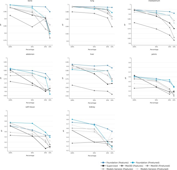
“More importantly, it remained robust as evidenced by the smallest decline in balanced accuracy and mAP of 9 and 12%, respectively, when reducing training data from 100 to 10%.”
§ Foundation model for cancer imaging biomarkers > Results > Pretraining strategy selection
boosteddirect- Asserted: passes — The authors put it forward as true.
- Checkable: passes — It can be checked against evidence.
- Load-bearing: passes — The paper’s conclusions depend on it.
- Based: passes — The paper gives a reason why it holds.
It may state two separate claims as one.
- Rests on an assumption: Following pretraining, foundation models can be applied to task-specific problems, improving generalization, especially in tasks with small datasets.
A result the paper reports from its own data — it cites no other source for it, so there is none to check. The quote shows it is in the paper.
In the paper
“Foundation (fine-tuned) showed a larger drop in performance and failed to improve significantly over baseline implementations as training data were decreased (losing significance from 20% onward).”
§ Foundation model for cancer imaging biomarkers > Results > Lesion anatomical site classification (use case 1)
plaindirectn = 1,010- Asserted: passes — The authors put it forward as true.
- Checkable: passes — It can be checked against evidence.
- Load-bearing: passes — The paper’s conclusions depend on it.
- Based: passes — The paper gives a reason why it holds.
It may state two separate claims as one.
- Rests on an assumption: Access to large amounts of annotated data for specialized applications is often challenging and demands expertise, time and labour.
- Rests on an assumption: The quantity and quality of annotated data are strongly linked to the robustness of deep-learning models.
The paper states this without a source or data behind it here, so there is nothing to check it against. The quote shows it is in the paper.
In the paper
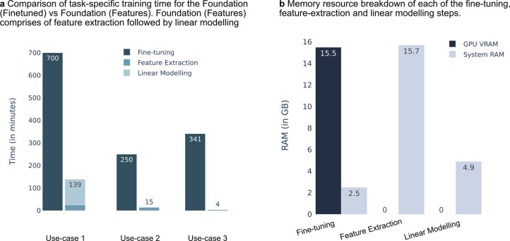
“Feature-based implementations were also computationally efficient when considering both time and memory.”
§ Foundation model for cancer imaging biomarkers > Discussion
plain- Asserted: passes — The authors put it forward as true.
- Checkable: passes — It can be checked against evidence.
- Load-bearing: fails — The paper’s conclusions may not depend on it.
- Based: passes — The paper gives a reason why it holds.
Probably not a substantial claim. The paper’s conclusions may not depend on it.
- Rests on an assumption: Access to large amounts of annotated data for specialized applications is often challenging and demands expertise, time and labour.
- Rests on an assumption: The quantity and quality of annotated data are strongly linked to the robustness of deep-learning models.
A result the paper reports from its own data — it cites no other source for it, so there is none to check. The quote shows it is in the paper.
In the paper
“For the RADIO cohort, Foundation (features) shows the best performance with an AUC of 0.653 (95% CI 0.532–0.771).”
§ Foundation model for cancer imaging biomarkers > Results > NSCLC prognostication (use case 3)
plaincorrelational- Asserted: passes — The authors put it forward as true.
- Checkable: passes — It can be checked against evidence.
- Load-bearing: passes — The paper’s conclusions depend on it.
- Based: passes — The paper gives a reason why it holds.
The quote only partly states this claim.
- Rests on an assumption: Access to large amounts of annotated data for specialized applications is often challenging and demands expertise, time and labour.
- Rests on an assumption: The quantity and quality of annotated data are strongly linked to the robustness of deep-learning models.
- Rests on an assumption: Image-biomarker studies for predicting endpoints such as overall survival on small cohorts largely rely on statistical feature extraction (engineered radiomics) and classical machine learning-based modelling.
- Rests on an assumption: These statistical feature extraction approaches require precise 3D segmentations, increasing the annotation burden of these studies.
A result the paper reports from its own data — it cites no other source for it, so there is none to check. The quote shows it is in the paper.
In the paper
“We found that absolute correlation coefficients between gene expression profiles and model predictions were significantly higher (P = 0.008) for the foundation model, indicating a stronger association with underlying tumour biology (Fig. 6a).”
§ Foundation model for cancer imaging biomarkers > Results > Underlying biological basis of the foundation model
hedgedcorrelationaln = 130 ·- Asserted: passes — The authors put it forward as true.
- Checkable: passes — It can be checked against evidence.
- Load-bearing: passes — The paper’s conclusions depend on it.
- Based: passes — The paper gives a reason why it holds.
It may state two separate claims as one.
A result the paper reports from its own data — it cites no other source for it, so there is none to check. The quote shows it is in the paper.
In the paper
“Modelling using features extracted from the foundation model was the most robust across these use cases when subjected to drops in training data, offering stable performance even when data sizes were considerably reduced, for example, using only 51 samples in use case 2.”
§ Foundation model for cancer imaging biomarkers > Discussion
plaincorrelationaln = 51- Asserted: passes — The authors put it forward as true.
- Checkable: passes — It can be checked against evidence.
- Load-bearing: passes — The paper’s conclusions depend on it.
- Based: passes — The paper gives a reason why it holds.
It may state two separate claims as one.
- Rests on an assumption: Access to large amounts of annotated data for specialized applications is often challenging and demands expertise, time and labour.
- Rests on an assumption: The quantity and quality of annotated data are strongly linked to the robustness of deep-learning models.
A result the paper reports from its own data — it cites no other source for it, so there is none to check. The quote shows it is in the paper.
In the paper
“When limited data (50, 20 and 10%) was used for downstream task training, our method demonstrated consistently improved performance.”
§ Foundation model for cancer imaging biomarkers > Results > Pretraining strategy selection
boosteddirect- Asserted: passes — The authors put it forward as true.
- Checkable: passes — It can be checked against evidence.
- Load-bearing: passes — The paper’s conclusions depend on it.
- Based: passes — The paper gives a reason why it holds.
The quote only partly states this claim.
- Rests on an assumption: Following pretraining, foundation models can be applied to task-specific problems, improving generalization, especially in tasks with small datasets.
A result the paper reports from its own data — it cites no other source for it, so there is none to check. The quote shows it is in the paper.
In the paper
“As expected, the second best-performing approach was SimCLR (balanced accuracy 0.696 (95% CI 0.663–0.728); mAP = 0.779 (95% CI 0.749–0.811)).”
§ Foundation model for cancer imaging biomarkers > Results > Pretraining strategy selection
plain- Asserted: passes — The authors put it forward as true.
- Checkable: passes — It can be checked against evidence.
- Load-bearing: unclear — It is unclear whether the paper’s conclusions depend on it.
- Based: passes — The paper gives a reason why it holds.
It may state two separate claims as one.
- Rests on an assumption: Following pretraining, foundation models can be applied to task-specific problems, improving generalization, especially in tasks with small datasets.
A result the paper reports from its own data — it cites no other source for it, so there is none to check. The quote shows it is in the paper.
In the paper
“We found that predictions from the overall best-performing models on LUNG1 and RADIO: Foundation (features) and Supervised (fine-tuned) had high stability with intraclass correlation coefficient (ICC) values of 0.984 and 0.966, respectively.”
§ Foundation model for cancer imaging biomarkers > Results > Stability of the foundation model
plainn = 26- Asserted: passes — The authors put it forward as true.
- Checkable: passes — It can be checked against evidence.
- Load-bearing: passes — The paper’s conclusions depend on it.
- Based: passes — The paper gives a reason why it holds.
It may state two separate claims as one.
A result the paper reports from its own data — it cites no other source for it, so there is none to check. The quote shows it is in the paper.
In the paper
“Foundation (fine-tuned) shows superior performance over all baselines at 50% but shows large drops in performance from a 20% reduction onward.”
§ Foundation model for cancer imaging biomarkers > Results > Nodule malignancy prediction (use case 2)
plaincorrelationaln = 254- Asserted: passes — The authors put it forward as true.
- Checkable: passes — It can be checked against evidence.
- Load-bearing: passes — The paper’s conclusions depend on it.
- Based: passes — The paper gives a reason why it holds.
It may state two separate claims as one.
- Rests on an assumption: Access to large amounts of annotated data for specialized applications is often challenging and demands expertise, time and labour.
- Rests on an assumption: The quantity and quality of annotated data are strongly linked to the robustness of deep-learning models.
The paper states this without a source or data behind it here, so there is nothing to check it against. The quote shows it is in the paper.
In the paper
“Furthermore, it surpasses current deep-learning techniques in various tasks while fitting conveniently into existing radiomic research methods.”
§ Foundation model for cancer imaging biomarkers > Discussion
plaindirect- Asserted: passes — The authors put it forward as true.
- Checkable: passes — It can be checked against evidence.
- Load-bearing: passes — The paper’s conclusions depend on it.
- Based: fails — The paper may give no reason why it holds.
Probably not a substantial claim. The paper may give no reason why it holds. It may state two separate claims as one.
The paper states this without a source or data behind it here, so there is nothing to check it against. The quote shows it is in the paper.
In the paper
“However, the original value of 0.1 proposed by the original paper was the most effective.”
§ Foundation model for cancer imaging biomarkers > Methods > Task-agnostic pretraining of the foundation model
plaindirect- Asserted: passes — The authors put it forward as true.
- Checkable: passes — It can be checked against evidence.
- Load-bearing: fails — The paper’s conclusions may not depend on it.
- Based: fails — The paper may give no reason why it holds.
Probably not a substantial claim. The paper’s conclusions may not depend on it. The paper may give no reason why it holds.
What the paper did — it cites no source for this, so there is none to check. The quote shows it is in the paper.
In the paper
“The baseline Models Genesis implementation was excluded in this analysis as this model was pretrained on the same dataset and, therefore, does not indicate a fair comparison.”
§ Foundation model for cancer imaging biomarkers > Results > Nodule malignancy prediction (use case 2)
plaindirect- Asserted: passes — The authors put it forward as true.
- Checkable: passes — It can be checked against evidence.
- Load-bearing: passes — The paper’s conclusions depend on it.
- Based: passes — The paper gives a reason why it holds.
Probably not a substantial claim. It may state two separate claims as one.
A conclusion the paper draws from its own results — it cites no other source for it, so there is none to check. The quote shows it is in the paper.
In the paper
“By contrast, our approach is generalizable to multiple use cases, and for nodule malignancy, we obtain high performance using significantly lesser training data, only 338 nodules (due to our more stringent exclusion criteria).”
§ Foundation model for cancer imaging biomarkers > Discussion
plaindirect- Asserted: passes — The authors put it forward as true.
- Checkable: passes — It can be checked against evidence.
- Load-bearing: passes — The paper’s conclusions depend on it.
- Based: passes — The paper gives a reason why it holds.
It may state two separate claims as one.
- Rests on an assumption: Access to large amounts of annotated data for specialized applications is often challenging and demands expertise, time and labour.
- Rests on an assumption: The quantity and quality of annotated data are strongly linked to the robustness of deep-learning models.
In the paper
“which is consistent with research demonstrating the tumour microenvironment’s influence on cancer development22 and prognosis.”
§ Foundation model for cancer imaging biomarkers > Results > Saliency maps for fine-tuned foundation models
What the sources say
- Not checked yetcites [22] Hinshaw, D. C. & Shevde, L. A. The tumor microenvironment innately modulates cancer progression. Cancer Res. 79, 4557–4566 (2019). source
boosteddirect- Asserted: passes — The authors put it forward as true.
- Checkable: passes — It can be checked against evidence.
- Load-bearing: fails — The paper’s conclusions may not depend on it.
- Based: passes — The paper gives a reason why it holds.
Probably not a substantial claim. The paper’s conclusions may not depend on it. It may state two separate claims as one.
A conclusion the paper draws from its own results — it cites no other source for it, so there is none to check. The quote shows it is in the paper.
In the paper
“as expressing saliency maps over 4,096-dimensional outputs remains challenging in practice.”
§ Foundation model for cancer imaging biomarkers > Methods > Feature visualization and saliency maps
plain- Asserted: passes — The authors put it forward as true.
- Checkable: passes — It can be checked against evidence.
- Load-bearing: passes — The paper’s conclusions depend on it.
- Based: fails — The paper may give no reason why it holds.
Probably not a substantial claim. The paper may give no reason why it holds.
A conclusion the paper draws from its own results — it cites no other source for it, so there is none to check. The quote shows it is in the paper.
In the paper
“This approach allows for significantly higher throughput than manual segmentation, which can be more tedious.”
§ Foundation model for cancer imaging biomarkers > Methods > Data preprocessing
plaindirect- Asserted: passes — The authors put it forward as true.
- Checkable: passes — It can be checked against evidence.
- Load-bearing: fails — The paper’s conclusions may not depend on it.
- Based: fails — The paper may give no reason why it holds.
Probably not a substantial claim. The paper’s conclusions may not depend on it. The paper may give no reason why it holds.
A conclusion the paper draws from its own results — it cites no other source for it, so there is none to check. The quote shows it is in the paper.
In the paper
“In conclusion, our foundation model offers a powerful and reliable framework for discovering cancer imaging biomarkers, especially in small datasets.”
§ Foundation model for cancer imaging biomarkers > Discussion
plaindirect- Asserted: passes — The authors put it forward as true.
- Checkable: passes — It can be checked against evidence.
- Load-bearing: passes — The paper’s conclusions depend on it.
- Based: fails — The paper may give no reason why it holds.
Probably not a substantial claim. The paper may give no reason why it holds.
In the paper
“Existing literature12 has suggested several strategies, such as image reconstruction, to pretrain networks to learn these representations.”
§ Foundation model for cancer imaging biomarkers > Main
What the sources say
- Not checked yetcites [12] Balestriero, R. et al. A cookbook of self-supervised learning. Preprint at https://arxiv.org/abs/2304.12210 (2023).
hedgeddirect- Asserted: passes — The authors put it forward as true.
- Checkable: passes — It can be checked against evidence.
- Load-bearing: fails — The paper’s conclusions may not depend on it.
- Based: passes — The paper gives a reason why it holds.
Probably not a substantial claim. The paper’s conclusions may not depend on it.
In the paper
“This point largely depends on the nature and sizes of training data in the downstream task.”
§ Foundation model for cancer imaging biomarkers > Discussion
What the sources say
- Not checked yetcites Cole et al.38 Cole, E., Yang, X., Wilber, K., Aodha, O. M. & Belongie, S. When does contrastive visual representation learning work? In Proc. 2022 IEEE/CVF Conference on Computer Vision and Pattern Recognition (CVPR) 14755–14764 (IEEE, 2022). source
plaincorrelational- Asserted: passes — The authors put it forward as true.
- Checkable: passes — It can be checked against evidence.
- Load-bearing: fails — The paper’s conclusions may not depend on it.
- Based: passes — The paper gives a reason why it holds.
Probably not a substantial claim. The paper’s conclusions may not depend on it.
In the paper
“Deep-learning methods, in comparison, are robust to differences in acquisition and segmentation variability and provide improved performance10.”
§ Foundation model for cancer imaging biomarkers > Discussion
What the sources say
- Not checked yetcites [10] Hosny, A. et al. Deep learning for lung cancer prognostication: a retrospective multi-cohort radiomics study. PLoS Med. 15, e1002711 (2018). source
plaindirect- Asserted: passes — The authors put it forward as true.
- Checkable: passes — It can be checked against evidence.
- Load-bearing: passes — The paper’s conclusions depend on it.
- Based: passes — The paper gives a reason why it holds.
It may state two separate claims as one.
A conclusion the paper draws from its own results — it cites no other source for it, so there is none to check. The quote shows it is in the paper.
In the paper
“as it is typical to have inherently small sample sizes in such use cases when compared to task complexity due to study-specific inclusion criteria.”
§ Foundation model for cancer imaging biomarkers > Methods > Task-specific training of the foundation model
plaindirect- Asserted: passes — The authors put it forward as true.
- Checkable: passes — It can be checked against evidence.
- Load-bearing: passes — The paper’s conclusions depend on it.
- Based: fails — The paper may give no reason why it holds.
Probably not a substantial claim. The paper may give no reason why it holds.
A conclusion the paper draws from its own results — it cites no other source for it, so there is none to check. The quote shows it is in the paper.
In the paper
“Third, a significant challenge with deep-learning models, including ours, is their ‘black box’ nature, which limits interpretability and explainability.”
§ Foundation model for cancer imaging biomarkers > Discussion
plaindirect- Asserted: passes — The authors put it forward as true.
- Checkable: passes — It can be checked against evidence.
- Load-bearing: fails — The paper’s conclusions may not depend on it.
- Based: passes — The paper gives a reason why it holds.
Probably not a substantial claim. The paper’s conclusions may not depend on it.
A conclusion the paper draws from its own results — it cites no other source for it, so there is none to check. The quote shows it is in the paper.
In the paper
“In our study, we pretrained on 11,467 lesion volumes and randomly sampled volumes, from 5,513 unique CT scans, leveraging not only one of the largest lesion-specific datasets but also one of the largest pretraining 3D CT datasets.”
§ Foundation model for cancer imaging biomarkers > Discussion
plain- Asserted: passes — The authors put it forward as true.
- Checkable: passes — It can be checked against evidence.
- Load-bearing: passes — The paper’s conclusions depend on it.
- Based: passes — The paper gives a reason why it holds.
It may state two separate claims as one.
None of the sources cited for this claim have been checked yet.
In the paper
“While many studies investigating imaging-based biomarkers incorporate supervised deep-learning algorithms into their models9–11, they are typically applied in scenarios where large datasets are available for training and testing.”
§ Foundation model for cancer imaging biomarkers > Main
What the sources say
- Not checked yetcites [9] Mahajan, A. et al. Deep learning-based predictive imaging biomarker model for EGFR mutation status in non-small cell lung cancer from CT imaging. J. Clin. Orthod. 38, 3106 (2020).
- Not checked yetcites [10] Hosny, A. et al. Deep learning for lung cancer prognostication: a retrospective multi-cohort radiomics study. PLoS Med. 15, e1002711 (2018). source
- Not checked yetcites [11] Braghetto, A., Marturano, F., Paiusco, M., Baiesi, M. & Bettinelli, A. Radiomics and deep learning methods for the prediction of 2-year overall survival in LUNG1 dataset. Sci. Rep. 12, 14132 (2022). source
plaincorrelational- Asserted: passes — The authors put it forward as true.
- Checkable: passes — It can be checked against evidence.
- Load-bearing: passes — The paper’s conclusions depend on it.
- Based: passes — The paper gives a reason why it holds.
It may state two separate claims as one.
In the paper
“They show a saturation point associated with pretraining dataset size and diminishing returns beyond this point.”
§ Foundation model for cancer imaging biomarkers > Discussion
What the sources say
- Not checked yetcites Cole et al.38 Cole, E., Yang, X., Wilber, K., Aodha, O. M. & Belongie, S. When does contrastive visual representation learning work? In Proc. 2022 IEEE/CVF Conference on Computer Vision and Pattern Recognition (CVPR) 14755–14764 (IEEE, 2022). source
plaincorrelational- Asserted: passes — The authors put it forward as true.
- Checkable: passes — It can be checked against evidence.
- Load-bearing: passes — The paper’s conclusions depend on it.
- Based: passes — The paper gives a reason why it holds.
Probably not a substantial claim.
What the paper did — it cites no source for this, so there is none to check. The quote shows it is in the paper.
In the paper
“In our comparative analysis, we maintained uniformity in batch sizes and dataset parameters across all methods, while optimizer and loss-specific settings were aligned with each method’s original configuration.”
§ Foundation model for cancer imaging biomarkers > Methods > Task-agnostic pretraining of the foundation model
plain- Asserted: passes — The authors put it forward as true.
- Checkable: passes — It can be checked against evidence.
- Load-bearing: fails — The paper’s conclusions may not depend on it.
- Based: passes — The paper gives a reason why it holds.
Probably not a substantial claim. The paper’s conclusions may not depend on it. It may state two separate claims as one.
A conclusion the paper draws from its own results — it cites no other source for it, so there is none to check. The quote shows it is in the paper.
In the paper
“Furthermore, our initial biological association analysis, aimed at explaining the model’s decisions, is preliminary and requires more rigorous investigation for a concrete understanding.”
§ Foundation model for cancer imaging biomarkers > Discussion
plain- Asserted: passes — The authors put it forward as true.
- Checkable: fails — It may be too vague to check against evidence.
- Load-bearing: fails — The paper’s conclusions may not depend on it.
- Based: passes — The paper gives a reason why it holds.
Probably not a substantial claim. It may be too vague to check against evidence. The paper’s conclusions may not depend on it.
A conclusion the paper draws from its own results — it cites no other source for it, so there is none to check. The quote shows it is in the paper.
In the paper
“due to the high proportion of negatives relative to positives, which results in consistently low false-positive rates and might overestimate the AUC.”
§ Foundation model for cancer imaging biomarkers > Methods > Performance analysis
hedgedconditional- Asserted: passes — The authors put it forward as true.
- Checkable: passes — It can be checked against evidence.
- Load-bearing: passes — The paper’s conclusions depend on it.
- Based: passes — The paper gives a reason why it holds.
It may state two separate claims as one.
None of the sources cited for this claim have been checked yet.
In the paper
“Several studies23–25 have demonstrated the efficacy of SSL in medicine where only limited data might be available for training deep-learning networks.”
§ Foundation model for cancer imaging biomarkers > Discussion
What the sources say
- Not checked yetcites [23] Azizi, S. et al. Big self-supervised models advance medical image classification. In 2021 IEEE/CVF International Conference on Computer Vision (ICCV) 3458–3468 (IEEE, 2021). source
- Not checked yetcites [24] Krishnan, R., Rajpurkar, P. & Topol, E. J. Self-supervised learning in medicine and healthcare. Nat. Biomed. Eng. 6, 1346–1352 (2022). source
- Not checked yetcites [25] Ghesu, F. C. et al. Contrastive self-supervised learning from 100 million medical images with optional supervision. J. Med. Imaging 9, 064503 (2022). source
boosteddirect- Asserted: passes — The authors put it forward as true.
- Checkable: passes — It can be checked against evidence.
- Load-bearing: fails — The paper’s conclusions may not depend on it.
- Based: passes — The paper gives a reason why it holds.
Probably not a substantial claim. The paper’s conclusions may not depend on it.
None of the sources cited for this claim have been checked yet.
In the paper
“We used scans from 26 patients from the RIDER dataset19, routinely used for test–retest robustness analysis in tumour imaging19–21.”
§ Foundation model for cancer imaging biomarkers > Results > Stability of the foundation model
What the sources say
- Not checked yetcites [19] Zhao, B. et al. Evaluating variability in tumor measurements from same-day repeat CT scans of patients with non-small cell lung cancer. Radiology 252, 263–272 (2009). source
- Not checked yetcites [20] Aerts, H. J. W. L. et al. Decoding tumour phenotype by noninvasive imaging using a quantitative radiomics approach. Nat. Commun. 5, 4006 (2014). source
- Not checked yetcites [21] Hosny, A. et al. Clinical validation of deep learning algorithms for radiotherapy targeting of non-small-cell lung cancer: an observational study. Lancet Digit. Health 4, e657–e666 (2022). source
plain- Asserted: passes — The authors put it forward as true.
- Checkable: passes — It can be checked against evidence.
- Load-bearing: fails — The paper’s conclusions may not depend on it.
- Based: passes — The paper gives a reason why it holds.
Probably not a substantial claim. The paper’s conclusions may not depend on it.
A conclusion the paper draws from its own results — it cites no other source for it, so there is none to check. The quote shows it is in the paper.
In the paper
“Therefore, experiments involving further data reduction in this case do not provide any valuable insights.”
§ Foundation model for cancer imaging biomarkers > Methods > Task-specific training of the foundation model
plain- Asserted: passes — The authors put it forward as true.
- Checkable: passes — It can be checked against evidence.
- Load-bearing: passes — The paper’s conclusions depend on it.
- Based: passes — The paper gives a reason why it holds.
Probably not a substantial claim.
The paper relies on this without support.
Access to large amounts of annotated data for specialized applications is often challenging and demands expertise, time and labour.
“However, access to large amounts of annotated data for specialized applications is often challenging and demands expertise, time and labour.”
The paper relies on this without support.
There is still limited evidence investigating whether SSL can help train foundation models that learn general, robust and transferrable representations that can act as imaging biomarkers, especially prognostic, for tasks of clinical relevance.
“There is still limited evidence investigating whether SSL can help train foundation models that learn general, robust and transferrable representations that can act as imaging biomarkers, especially prognostic, for tasks of clinical relevance.”
The paper relies on this without support.
The quantity and quality of annotated data are strongly linked to the robustness of deep-learning models.
“The quantity and quality of annotated data are strongly linked to the robustness of deep-learning models.”
The paper relies on this without support.
In scenarios with limited annotated data, many investigators fall back on traditional handcrafted or engineered approaches that limit the scope of discovery.
“In such scenarios, many investigators fall back on traditional handcrafted or engineered approaches based on defined mathematical and statistical algorithms that analyse attributes such as the shape and texture of objects in images, which limit the scope of discovery.”
The paper relies on this without support.
Following pretraining, foundation models can be applied to task-specific problems, improving generalization, especially in tasks with small datasets.
“Following pretraining, foundation models can be applied to task-specific problems, improving generalization, especially in tasks with small datasets.”
The paper relies on this without support.
Image-biomarker studies for predicting endpoints such as overall survival on small cohorts largely rely on statistical feature extraction (engineered radiomics) and classical machine learning-based modelling.
“Image-biomarker studies for predicting endpoints, such as overall survival on small cohorts, largely rely on statistical feature extraction (engineered radiomics) and classical machine learning-based modelling.”
The paper relies on this without support.
These statistical feature extraction approaches require precise 3D segmentations, increasing the annotation burden of these studies.
“These require precise 3D segmentations for feature extraction, increasing the annotation burden of these studies.”
Claims other papers make about this one
Each is checked against this paper’s own text: does it say what the citing paper says it does?
The cited source says what the claim attributes to it.
In the citing paper
“Built on rich knowledge representations, these models have shown impressive performance across medical fields such as ophthalmology20, radiology21 and pathology22–25.”
From A Multimodal Vision Foundation Model for Clinical Dermatology (2025) · cites this paper as [21]
In the citing paper
“In oncology, transformer-based methods support clinical text processing, whole-slide and radiologic image interpretation (vision transformers), and genomic sequence modeling [24,25,26,27].”
From Artificial Intelligence in Clinical Oncology: From Productivity Enhancement to Creative Discovery (2025) · cites this paper as [24]
In the citing paper
“Specialty-specific foundation models20,21,23 typically focus on single imaging modalities”
From A Multimodal Vision Foundation Model for Clinical Dermatology (2025) · cites this paper as [21]
Self-check
Percentages, sums and reported differences re-computed from the paper’s own numbers.
Each contradiction between two passages listed here was confirmed by an independent check.
Rated minor: it would not touch a result — a value no result rests on, a p-value that stays on the same side of the significance level, or a conflict that is clerical, resolved elsewhere in the paper, or outside its own findings.
In the paper
§ Foundation model for cancer imaging biomarkers > Results > Stability of the foundation model
“Each AUC and MSE measure in the box plots (d,e) have been computed on a dataset with n = 422 samples”
§ Foundation model for cancer imaging biomarkers > Methods > Study population
“For our study, we selected CT scans of 420 patients (right-censored for 2-year survival) with annotated primary gross tumour volumes and used these as an independent test set for prognostication networks.”
Rated minor: it would not touch a result — a value no result rests on, a p-value that stays on the same side of the significance level, or a conflict that is clerical, resolved elsewhere in the paper, or outside its own findings.
In the paper
§ Foundation model for cancer imaging biomarkers > Results > Pretraining strategy selection
“mAP = 0.847”
§ Foundation model for cancer imaging biomarkers > Results > Pretraining strategy selection
“95% CI 0.750–0.810”
Citations
Cites
Deep Residual Learning for Image Recognition
He, K., Zhang, X., Ren, S., & Sun, J. (2016) · 2016 IEEE Conference on Computer Vision and Pattern Recognition (CVPR) · doi:10.1109/cvpr.2016.90 · Cited by 235,474
Learning Transferable Visual Models From Natural Language Supervision
Radford, A., Kim, J. W., Hallacy, C., Ramesh, A., Goh, G., Agarwal, S., Sastry, G., Askell, A., Mishkin, P., Clark, J., et al. (2021) · arXiv · doi:10.48550/arxiv.2103.00020 · Cited by 15,293
Larian Studios Dev Team (2024) · doi:10.1145/3292500.3330701 · Cited by 8,618
Decoding tumour phenotype by noninvasive imaging using a quantitative radiomics approach
Aerts, H. J. W. L., Velazquez, E. R., Leijenaar, R. T. H., Parmar, C., Grossmann, P., Carvalho, S., Bussink, J., Monshouwer, R., Haibe-Kains, B., Rietveld, D., et al. (2014) · Nature Communications · doi:10.1038/ncomms5006 · Cited by 5,132
Self-citationTraining language models to follow instructions with human feedback
Ouyang, L., Wu, J., Jiang, X., Almeida, D., Wainwright, C. L., Mishkin, P., Zhang, C., Agarwal, S., Slama, K., Ray, A., et al. (2022) · arXiv · doi:10.48550/arxiv.2203.02155 · Cited by 4,208
The Tumor Microenvironment Innately Modulates Cancer Progression
Hinshaw, D. C., & Shevde, L. A. (2019) · Cancer Research · doi:10.1158/0008-5472.can-18-3962 · Cited by 3,270
On the Opportunities and Risks of Foundation Models
Bommasani, R., Hudson, D. A., Adeli, E., Altman, R., Arora, S., von Arx, S., Bernstein, M. S., Bohg, J., Bosselut, A., Brunskill, E., et al. (2021) · arXiv · doi:10.48550/arxiv.2108.07258 · Cited by 2,676
Unsupervised Learning of Visual Features by Contrasting Cluster Assignments
Caron, M., Misra, I., Mairal, J., Goyal, P., Bojanowski, P., & Joulin, A. (2020) · arXiv · doi:10.48550/arxiv.2006.09882 · Cited by 2,499
Foundation models for generalist medical artificial intelligence
Moor, M., Banerjee, O., Abad, Z. S. H., Krumholz, H. M., Leskovec, J., Topol, E. J., & Rajpurkar, P. (2023) · Nature · doi:10.1038/s41586-023-05881-4 · Cited by 2,028
SmoothGrad: removing noise by adding noise
Smilkov, D., Thorat, N., Kim, B., Viégas, F., & Wattenberg, M. (2017) · arXiv · doi:10.48550/arxiv.1706.03825 · Cited by 1,467
Research works printed but not linked: 8
- Devlin, J., Chang, M.-W., Lee, K. & Toutanova, K. BERT: Pre-training of deep bidirectional transformers for language understanding. In Proc. 2019 Conference of the North American Chapter of the Association for Computational Linguistics (eds Burstein, J. et al.) 4171–4186 (ACL, 2019).
- Chen, T., Kornblith, S., Norouzi, M. & Hinton, G. A simple framework for contrastive learning of visual representations. In Proc. 37th International Conference on Machine Learning (eds III, H.D. & Singh, A.) 1597–1607 (PMLR, 2020).
- Kumar, D. et al. in Image Analysis and Recognition (eds Karray, F. et al.) 54–62 (Springer, 2017).
- Taleb, A. et al. 3D self-supervised methods for medical imaging. Adv. Neural Inf. Process. Syst. 33, 18158–18172 (2020).
- Adebayo, J. et al. Sanity checks for saliency maps. In Advances in Neural Information Processing Systems 9505–9515 (Curran Associates, 2018).
- Sohn, K. Improved deep metric learning with multi-class N-pair loss objective. In Advances in Neural Information Processing Systems (eds Lee, D. et al.) 1857–1865 (Curran Associates, 2016).
- van der Maaten, L. & Hinton, G. Visualizing data using t-SNE. J. Mach. Learn. Res. 9, 2579–2605 (2008).
- Springenberg, J. T., Dosovitskiy, A., Brox, T. & Riedmiller, M. A. Striving for simplicity: the all convolutional net. In 3rd International Conference on Learning Representations Workshop (ICLR, 2015).
Cited by
Sorted by citations
Items 101–199 of 199
Feature Copy-Paste Network for Lung Cancer EGFR Mutation Status Prediction in CT Images
Huang, X., Wang, S., Liu, C., et al. (2025) · Lecture notes in computer science · doi:10.1007/978-3-032-05182-0_21 · Cited by 2
Clinical knowledge enhanced medical image classification
Xu, Z., Liang, J., Wei, Z., Yue, X., & Li, D. (2025) · Pattern Recognition · doi:10.1016/j.patcog.2025.112414 · Cited by 2
Ma, D., Pang, J., Velan, S. S., Gotway, M. B., & Liang, J. (2025) · Medical Image Analysis · doi:10.1016/j.media.2025.103828 · Cited by 5
Hu, M., Hu, X., Chen, W., Xia, C., Yao, W., Zuo, M., Lin, Z., Deng, L., & Wu, Z. (2025) · Scientific Reports · doi:10.1038/s41598-025-26331-3 · Cited by 3
Petrochuk, J., Pai, S., He, J., Haugg, F., Xu, Y., Christiani, D. C., Mak, R. H., & Aerts, H. J. W. L. (2025) · Scientific Reports · doi:10.1038/s41598-025-26365-7 · Cited by 3
Self-citationShiokawa, R., Iwasawa, J., Tanaka, Y., Tokuoka, Y., Sugawara, Y., Hirano, Y., Takaji, R., Hayakawa, Y. K., Oda, K., Kudo, Y., et al. (2025) · Scientific Reports · doi:10.1038/s41598-025-30277-x · Cited by 2
Predicting lung cancer survival with attention-based CT slices combination
Paolo, D., Greco, C., Ippolito, E., Fiore, M., Ramella, S., Soda, P., Tortora, M., Bria, A., & Sicilia, R. (2026) · Health Information Science and Systems · doi:10.1007/s13755-025-00404-z · Cited by 3
Multi-omics fusion network for prediction of early recurrence in colorectal liver metastases
Saber, R., Carneiro, M., Montagnon, E., Tang, A., Turcotte, S., & Kadoury, S. (2026) · npj Precision Oncology · doi:10.1038/s41698-025-01264-2 · Cited by 2
Kuang, S., Schuitmaker, L., Wu, M., Salahuddin, Z., van der Wiel, A. M.-M. A., van de Laak, J., Lieuwes, N. G., Biemans, R., Jung, J., Yaromina, A., et al. (2026) · npj Precision Oncology · doi:10.1038/s41698-026-01322-3 · Cited by 2
Foundation models in medical imaging: A review
Chen, Q., Liu, A., Zhang, J., Yang, C., & Zhang, Y. (2026) · EngMedicine · doi:10.1016/j.engmed.2026.100123 · Cited by 8
Petti, D. J., Li, C., & Liu, N. (2026) · Plant Phenomics · doi:10.1016/j.plaphe.2026.100193 · Cited by 2
Overview of State-of-the-Art Learning-Based Classification Methods in Medical Imaging
Nia, N. G., Manwar, R., & Avanaki, K. (2026) · Annals of Biomedical Engineering · doi:10.1007/s10439-026-04241-3 · Cited by 2
Generative Artificial Intelligence and Large Language Models in Clinical Oncology
Yu, Y., Zhao, Z., Wang, Z., Lin, R., Tan, Y., Chen, Y., Li, T., Baptista‐Hon, D. T., Zhang, X., Wu, C., et al. (2026) · MedComm · doi:10.1002/mco2.70833 · Cited by 2
MerMED-FM: Multimodal, Multi-Disease Medical Imaging Foundation Model
Zhou, Y., Quek, C. W. N., Zhou, J., Wang, Y., Bai, Y., Gutiérrez, L., Ke, Y., Yao, J., Teo, Z. L., Ting, D. S. J., et al. (2026) · The Lancet Digital Health · doi:10.1016/j.landig.2026.101007 · Cited by 2
Yue, Q., Zhang, M., Jiang, W., et al. (2024) · BMC Cancer · doi:10.1186/s12885-024-13149-x · Cited by 2
Zhang, T., Liang, X., & Mann, R. M. (2025) · European Radiology · doi:10.1007/s00330-025-12085-z · Cited by 2
A comprehensive foundation model for cryo-EM image processingPreprint
Yang, Y. X., Fan, S., Yuan, F., et al. (2024) · bioRxiv (Cold Spring Harbor Laboratory) · doi:10.1101/2024.11.04.621604 · Cited by 2
A Multimodal Vision-text AI Copilot for Brain Disease Diagnosis and Medical ImagingPreprint
Zhang, G., Gao, Z., Duan, C., Liu, J., Lizhu, Y., Liu, Y., Chen, Q., Wang, L., Fei, K., Wang, T., et al. (2025) · medRxiv · doi:10.1101/2025.01.09.25320293 · Cited by 6
Graph Neural Networks: A Suitable Alternative to MLPs in Latent 3D Medical Image Classification?
Kiechle, J., Lang, D. M., Fischer, S. M., et al. (2025) · Lecture notes in computer science · doi:10.1007/978-3-031-83243-7_2 · Cited by 3
Zhuang, L., Tabatabaei, S. M. H., Aberle, D. R., et al. (2025) · doi:10.1117/12.3049090 · Cited by 1
The Expanding Landscape of Neural Architectures and Their Impact in Biomedicine
Zhang, Z. F., Zhan, H., Wu, T., Burns, R., Hundal, J., & Costa, H. A. (2025) · Annual Review of Biomedical Data Science · doi:10.1146/annurev-biodatasci-103023-050856 · Cited by 1
Masquelin, A. H. P., & Estépar, R. S. J. (2025) · Lecture notes in computer science · doi:10.1007/978-3-032-05169-1_47 · Cited by 1
Anatomy-informed deep learning and radiomics for neurofibroma segmentation in whole-body MRI
Kolokolnikov, G., Schmalhofer, M., Well, L., et al. (2025) · Computerized Medical Imaging and Graphics · doi:10.1016/j.compmedimag.2025.102667 · Cited by 1
Precise leaf damage detection across diverse species and environments via a large-scale vision model
Chen, W., Ruan, H., Zhou, P., He, L., & 阮新潮 (2026) · Frontiers in Plant Science · doi:10.3389/fpls.2026.1788926 · Cited by 1
Clinical Implementation of Artificial Intelligence Systems in Medical Imaging and Radiotherapy
Vienna International Centre, 100, P. B., Vienna, A.-1., Austria, 2600-0, T. +. (., & 2600-7, F. +. (. (2026) · IAEA human health series · doi:10.61092/iaea.9olq-aqa9 · Cited by 2
Tables Guide Vision: Learning to See the Heart through Tabular Data
Hasny, M., Folco, M. D., Bressem, K. K., & Schnabel, J. A. (2026) · IEEE Winter Conference on Applications of Computer Vision · doi:10.1109/wacv61042.2026.00172 · Cited by 3
Ji, J., Zhang, X., Hua, M., Wang, M., Li, H., Zheng, X., Wang, L., Wang, H., Song, Y., He, J., et al. (2026) · npj Precision Oncology · doi:10.1038/s41698-026-01449-3 · Cited by 1
Haraldsson, A., Askmyr, D., Altunbulakli, C., Nilsson, M. G., Pignol, J., Gustafsson, C. J., Linnér, A., Lindstedt, M., Greiff, L., & Gebre-Medhin, M. (2026) · Radiotherapy and Oncology · doi:10.1016/j.radonc.2026.111607 · Cited by 1
Pozzi, J., D’Argenzio, J., Carriero, S., Cè, M., D’Arrigo, D., Lanza, C., Biondetti, P., Angileri, S. A., Pavan, M., Catona, R., et al. (2026) · Diagnostics · doi:10.3390/diagnostics16142266 · Cited by 2
Machine Learning for Radiomics in Oncology: Challenges, Limitations, and Future Directions
Missaoui, R., Saadaoui, W., Coco, M. D., Helali, A., Leo, M., & Carcagnì, P. (2026) · Sensors · doi:10.3390/s26144619 · Cited by 2
Corso, F., Zec, A., Favali, M., Ligero, M., Hilgers, L., Invernizzi, L. M., Mazzeo, L., Morales, A. M., Müller‐Franzes, G. A., Machado, I. P., et al. (2026) · Cell Reports Medicine · doi:10.1016/j.xcrm.2026.102966 · Cited by 2
Prelaj, A., Miskovic, V., Sacco, M., Ferrarin, A., Licciardello, C. M., Provenzano, L., Favali, M., Lerma, L., Zec, A., Spagnoletti, A., et al. (2026) · Nature Medicine · doi:10.1038/s41591-026-04488-2 · Cited by 2
AI4Skeletons: bringing in a new era of the digital intelligent skeleton with artificial intelligence
Wang, L., Wang, W., Liu, Y., Glüer, C.-C., Zhang, Y., & Liu, Y. (2025) · 中国科学通报:英文版 · doi:10.1016/j.scib.2025.04.057 · Cited by 1
Erdur, A. C., Scholz, D., Nguyen, Q. M., Buchner, J. A., Mayinger, M. C., Christ, S. M., Brunner, T. B., Wittig, A., Zimmer, C., Meyer, B., et al. (2025) · Radiotherapy and Oncology · doi:10.1016/j.radonc.2025.111031 · Cited by 2
Training-free Design of Deep Networks as Ensembles of Clinical ExpertsPreprint
Wu, T., Wu, J., Zhang, Z., & Chen, W. (2024) · medRxiv · doi:10.1101/2024.03.17.24304438 · Cited by 1
A New Foundation Model’s Accuracy in Glaucoma Detection using Ocular Coherence Tomography ImagesPreprint
Chuter, B., Huynh, J., Walker, E., Hallaj, S., Jalili, J., Liebmann, J. M., Fazio, M. A., Girkin, C. A., Weinreb, R. N., Christopher, M. A., et al. (2024) · medRxiv · doi:10.1101/2024.08.04.24311475 · Cited by 1
Foundation model embeddings for quantitative tumor imaging biomarkersPreprint
Pai, S., Hadžić, I., Fedorov, A., Mak, R. H., & Aerts, H. J. W. L. (2025) · Research Square · doi:10.21203/rs.3.rs-6630446/v1 · Cited by 1
Self-citationThymus Composition, Disease Control, and Toxicity in Locally Advanced Lung CancerPreprint
Chaunzwa, T. L., Book, A. J., Garomsa, B. A., Meng, Y. J., Yang, E., Krishnan, G., Chidi, A. P., Kim, H. R., Ma, J., Riely, G. J., et al. (2025) · medRxiv · doi:10.1101/2025.10.20.25338395 · Cited by 1
Self-citationREECAP: Contrastive learning of retinal aging reveals genetic loci linking morphology to eye diseasePreprint
Shilova, L., Sens, D., Aliyeva, A., Chaudhary, S., Xu, Q., Salin, E., Schiefelbein, J. B., Asani, B., Amarie, O. V., Schneltzer, E., et al. (2025) · medRxiv · doi:10.1101/2025.11.19.25340555 · Cited by 2
Evaluation of Spatially Variable Genes as Biomarkers in Tumor Initiation and Progression
Uzunoğlu, A. S., Uzunoğlu, M. S., Çapuk, S., & Taş, S. K. (2024) · Advances in medical diagnosis, treatment, and care (AMDTC) book series · doi:10.4018/979-8-3693-7728-4.ch003
Meneghetti, A. R., Ligero, M., Kuehn, J.-P., et al. (2025) · medRxiv · doi:10.1101/2025.01.22.25320517
Automated diagnosis of usual interstitial pneumonia on chest CT via the mean curvature of isophotesPreprint
Savadjiev, P., Rezanejad, M., Bhatnagar, S., et al. (2025) · medRxiv · doi:10.1101/2025.02.28.25322740
Park, S. H., Yadav, A., Tabatabaei, H., Lin, Y., Aberle, D. R., Prosper, A. E., & Hsu, W. W. Y. (2025) · SPIE Medical Imaging: Imaging Informatics for Healthcare, Research, and Applications · doi:10.1117/12.3049089
Su, F., Yi, X., Ye, C., et al. (2025) · medRxiv · doi:10.1101/2025.04.12.25325728
Informatics at the Frontier of Cancer Research
Noller, K., Botsis, T., Cámara, P. G., Ciotti, L., Cooper, L., Goecks, J., Griffith, M., Haas, B. J., Ideker, T., Karchin, R., et al. (2025) · Cancer Research · doi:10.1158/0008-5472.can-24-2829 · Cited by 2
Lighter: Configuration-Driven Deep Learning
Hadžić, I., Pai, S., Bressem, K. K., et al. (2025) · The Journal of Open Source Software · doi:10.21105/joss.08101
Self-citationDeep learning models for deriving optimised measures of fat and muscle mass from MRI
Thomas, B., Ali, M., Ali, F. M. H., Chung, A. J.-Y., Joshi, M., Maiguma-Wilson, S., Reiff, G., Said, H., Zalmay, P., Berks, M., et al. (2025) · Scientific Reports · doi:10.1038/s41598-025-07867-w
Kuang, S., Schuitmaker, L., Wu, M., Salahuddin, Z., van der Wiel, A. M.-M. A., van de Laak, J., Lieuwes, N. G., Biemans, R., Jung, J., Yaromin, A., et al. (2025) · SSRN Electronic Journal · doi:10.2139/ssrn.5381282
Lopukhova, E. A., Yusupov, E. S., Ibragimova, R. R., Маратовна, И. Г., Рафаэльевич, М. Т., Grakhova, E. P., & Kutluyarov, R. V. (2025) · Applied Sciences · doi:10.3390/app151810197
Abnormality-Driven Representation Learning for Radiology Imaging
Ligero, M., Lenz, T., Wölflein, G., Nahhas, O. S. M. E., Truhn, D., & Kather, J. N. (2025) · Lecture notes in computer science · doi:10.1007/978-3-032-04965-0_2
More than meets the eye: decoding glioma genomes in MRI pixel patterns
Li, Z., Liang, D., & Zheng, H. (2025) · European Radiology · doi:10.1007/s00330-025-12041-x
Radiomics-based intelligent diagnosis and treatment
Fang, M., Wang, Z., Fu, J., Wang, Y., Zhao, Y., Qin, Z., Zhang, C., Xie, X., Tang, L., & Dong, D. (2025) · Elsevier eBooks · doi:10.1016/b978-0-443-30142-1.00006-7
Leveraging Artificial Intelligence to Transform Thoracic Radiology for Lung Nodules and Lung Cancer
Lee, G., Cho, H.-H., Jeong, D. Y., Kim, J., Oh, Y. J., Park, S. G., & Lee, H. Y. (2025) · Journal of Thoracic Imaging · doi:10.1097/rti.0000000000000866 · Cited by 1
Ji, X., Dong, S., Shen, Z., Pu, Y., Zou, X., Xia, W., & Li, R. (2025) · ICME International Conference on Complex Medical Engineering (CME) · doi:10.1109/cme67420.2025.11239374
Trustworthy assessment of 2D model for lung CT scans
Favali, M., Miskovic, V., Eusebio, A., Trovò, F., Provenzano, L., Guirges, B., Ruggirello, M., Garassino, M. C., Proto, C., Russo, G. L., et al. (2025) · Annual International Conference of the IEEE Engineering in Medicine and Biology Society (EMBC) · doi:10.1109/embc58623.2025.11254399
Automated diagnosis of usual interstitial pneumonia on chest CT via the mean curvature of isophotes
Savadjiev, P., Rezanejad, M., Bhatnagar, S., Camirand, D., Kauffmann, C., Kaleem Siddiqi, A., Dandurand, R. J., Bourgouin, P., Chartrand‐Lefebvre, C., & Semionov, A. (2026) · European Journal of Radiology Open · doi:10.1016/j.ejro.2025.100723
CLEAR: An Auditable Foundation Model for Radiology Grounded in Clinical ConceptsPreprint
Han, T., Wu, R., Tian, Y. X., et al. (2026) · medRxiv · doi:10.64898/2026.01.15.26344222
I3LUNG: Clinical Validation of a Multimodal AI Tool to Support Immunotherapy Decisions in NSCLCPreprint
Prelaj, A., Miskovic, V., Sacco, M., Ferrarin, A., Licciardello, C. M., Provenzano, L., Favali, M., Lerma, L., Zec, A., Spagnoletti, A., et al. (2026) · medRxiv · doi:10.64898/2026.01.16.25342913
Established Machine Learning Matches Tabular Foundation Models in Clinical PredictionsPreprint
Shaktah, L., Gustav, M., Lenz, T., Liang, J., Hilgers, L., Carrero, Z. I., & Kather, J. N. (2026) · medRxiv · doi:10.64898/2026.02.02.26345274
Kanapeckaitė, A., Peters, C. J., Laurinavičius, A., & Geris, L. (2025) · Integrative Biology · doi:10.1093/intbio/zyaf024
A multimodal embedding model for sepsis data representation
Liu, T., Li, Y., Chen, H., Li, N., Zhang, Y., Huang, X., Wang, J., Chen, R., Zeng, Y., Liu, Y., et al. (2026) · npj Digital Medicine · doi:10.1038/s41746-026-02446-3 · Cited by 1
Abstract: Physiological Neural Representations in Dynamic Imaging
Tehlan, K., & Wendler, T. (2026) · Informatik aktuell · doi:10.1007/978-3-658-51100-5_69
Kolokolnikov, G., Schmalhofer, M., Well, L., et al. (2026) · Informatik aktuell · doi:10.1007/978-3-658-51100-5_48
Leveraging single-cell foundation models for accurate survival outcome prediction
Liu, W., Wang, Q., Long, L., & Wang, W. (2026) · Bioinformatics Advances · doi:10.1093/bioadv/vbag076 · Cited by 1
Cross-Scanner Reliability of Brain MRI Foundation Model Embeddings: A Travelling-Heads StudyPreprint
González, R. N., Aja‐Fernández, S., Planchuelo‐Gómez, Á., & de Luis-Garcı́a, R. (2026) · medRxiv · doi:10.64898/2026.03.23.26348808
Advancing Lung Cancer Imaging with Self-Supervised Foundation Models
Varona, D. (2026) · Radiology Imaging Cancer · doi:10.1148/rycan.260078
Label-free digital protein sensing by integral plasmonic imaging
Sun, Y., Wang, J., Zeng, Q., et al. (2026) · Fundamental Research · doi:10.1016/j.fmre.2026.04.009
Fusing imaging and metabolic modeling via multimodal deep learning in ovarian cancer
Eftekhari, N., Verma, S., Saha, A., Zampieri, G., Sawan, S., Occhipinti, A., & Angione, C. (2026) · Cell Systems · doi:10.1016/j.cels.2026.101594
Biosensors-Immunoassay by ECL Imaging and Microscopy
Zheng, Y., Zholudov, Y. T., Snizhko, D. V., Muzyka, K., Guan, Y., & Xu, G. (2026) · Springer eBooks · doi:10.1007/978-3-032-14602-1_7 · Cited by 1
Ferle, M., Ader, J., Wiemers, T. C., Grieb, N., Berneck, B., Lindenmeyer, A., Goldschmidt, H., Mai, E. K., Bertsch, U., Meyer, H., et al. (2026) · npj Digital Medicine · doi:10.1038/s41746-026-02663-w
Zhao, C., Lai, S., He, J., et al. (2026) · Talanta · doi:10.1016/j.talanta.2026.129972
Gilbert, A., Gacad, A., Parrish, L., et al. (2026) · doi:10.2196/preprints.101509
Guo, R., Zhang, M., Zhu, H., Tang, X., Fu, W., Li, M., Hu, H. B., Xiao, X., Wang, W., Liu, Y., et al. (2026) · The Lancet Regional Health - Western Pacific · doi:10.1016/j.lanwpc.2026.101890 · Cited by 1
MHub.ai: A Standardized Platform for Reproducible AI Research in Medical ImagingPreprint
Aerts, H. J. W. L., Nürnberg, L., Bontempi, D., Pai, S., Lisle, C. R., Pieper, S., Kikinis, R., van de Leemput, S. C., Soni, R., Murugesan, G., et al. (2026) · Research Square · doi:10.21203/rs.3.rs-9480032/v1
Self-citationFelici, B., Chen, S., Yuan, M., Jiang, X., Ip, S. H. Y., Rudd, J. H. F., & Inouye, M. (2026) · Cell Genomics · doi:10.1016/j.xgen.2026.101282
CLEAR: an auditable foundation model for radiology grounded in clinical concepts
Han, T., Wu, R., Tian, Y., Khader, F., Adams, L. C., Bressem, K. K., Davatzikos, C. A., Kather, J. N., Shen, L., Mankoff, D. A., et al. (2026) · Nature Biomedical Engineering · doi:10.1038/s41551-026-01741-4 · Cited by 3
Shahzadi, I., & Borggrefe, J. (2026) · RöFo - Fortschritte auf dem Gebiet der Röntgenstrahlen und der bildgebenden Verfahren · doi:10.1055/a-2899-1290
Multi-source data-driven machine learning for lung cancer: diagnosis, treatment, and prognosis
Zou, Y., Zhu, J., Cheng, J., Yan, J., Dai, B., Han, J., & Guo, J. (2026) · Intelligent Opto-Electronics · doi:10.67704/ioe.2026.260006
Foundation Models Meet Digital Breast Tomosynthesis
Wu, S. (2026) · Radiology · doi:10.1148/radiol.261974
The Rise of Generalist Foundation Models and Quantum Computing in Oncology
Kakar, M. (2026) · Technology in Cancer Research & Treatment · doi:10.1177/15330338261476208
Yadav, K., & Gupta, T. (2026) · Journal of the Egyptian National Cancer Institute · doi:10.1186/s43046-026-00399-y
Chung, W., Park, Y., Kwak, Y., Lee, H. D., Kim, B., Shin, C. M., Nam, Y., & Lee, H. S. (2026) · Laboratory Investigation · doi:10.1016/j.labinv.2026.106161
AI-powered medicinal chemistry and translational drug development
Kaicheng, U., Zhang, S. M., Yu, Z., Zhang, Z., Zhang, J., He, C., Liu, A., Chen, R., Wang, S., Yan, L., et al. (2026) · Chemical Society Reviews · doi:10.1039/d5cs01469g
Systematic evaluation of foundation models for organ-level classification on CT scans
Tagscherer, J., de Boer, S., der Graaf, F. V., Philipp, L., Jacobs, C., Smit, E. J., & Hering, A. (2026) · International Journal of Computer Assisted Radiology and Surgery · doi:10.1007/s11548-026-03786-x
Yew, S. M. E., Lei, X., Goh, J. H. L., Zou, K., Chen, Y., Srinivasan, S., Chee, M.-L., Pushpanathan, K., Hou, Q., Soh, Z. D., et al. (2026) · The Lancet Digital Health · doi:10.1016/j.landig.2026.101031 · Cited by 2
Shao, J., Liu, X., Zhang, Z., Liao, S., Wu, J., Yang, H., Zhao, Z., Wang, L., Liang, S.-F., Wang, X., et al. (2026) · Cell Reports Medicine · doi:10.1016/j.xcrm.2026.102926
Digital Twins in Oncology: From Multimodal Data Integration to Precision Clinical Practice
Vairavan, A., Bhattacharjee, R., & Raghavan, B. (2026) · Indian journal of radiology and imaging - new series/Indian journal of radiology and imaging/Indian Journal of Radiology & Imaging · doi:10.1055/s-0046-1827804
Generative artificial intelligence technologies in pathology
Ullah, E. (2026) · Elsevier eBooks · doi:10.1016/b978-0-443-40383-5.00013-3
Wang, L., Shi, Y., Deng, Z., Wang, Y., Righi, D. R. D., Javed, S., Qureshi, T. A., Yang, J. D., Xie, Y., Pandol, S. J., et al. (2026) · Artificial Intelligence in Medicine · doi:10.1016/j.artmed.2026.103535
Solovev, I. A., & Golubev, D. (2026) · Real-World Data & Evidence · doi:10.37489/2782-3784-myrwd-114
Liu, C., Li, S., Sang, H., Huang, X., Wang, C., Shu, Y., Wu, Y., Tian, J., Zhang, H., Zhang, L., et al. (2026) · Visual Computing for Industry Biomedicine and Art · doi:10.1186/s42492-026-00233-1
Artificial intelligence in biomarker discovery for diseases: diagnostic and therapeutic prospects
Dinç, R., & Ardıç, N. (2026) · Signal Transduction and Targeted Therapy · doi:10.1038/s41392-026-02946-4 · Cited by 1
Personalized Healthcare for Cancers
Ali, K. A., Bishal, A., Choudhuri, S., Dutta, S., Das, T., & Roy, S. K. (2026) · IGI Global eBooks · doi:10.4018/979-8-3373-9715-3.ch002
Lin, H., Huang, B., Wang, M., Ren, Y., Liu, Z., & Huang, B. (2026) · Lecture notes in computer science · doi:10.1007/978-3-032-38470-6_58
Wijaya, J. H., Gillam, W. B., V, Lamprecht, C. B., Ruchika, F., Schneider, B., Foster, D., Abolfazli, P., Perez-Chadid, D. A., Azmi, A., Madrigal, J. P. Á., et al. (2026) · Journal of Imaging Informatics in Medicine · doi:10.1007/s10278-026-02290-7
AI-Enabled Digital Health Tool Implementation in Clinical Practice Settings: Umbrella Review
Gilbert, A. S., Gacad, A., Parrish, L. J., Nguyen, O. T., Turner, K. L., Tarver, W. L., Jonnalagadda, P., Tsagli, D. D., Wu, B., Lu, C., et al. (2026) · JMIR AI · doi:10.2196/101509
Nakano, H., & Shiinoki, T. (2026) · Journal of Imaging Informatics in Medicine · doi:10.1007/s10278-026-02344-w
Generative AI versus physicians in diagnostic radiology: a systematic review and meta-analysis
Takita, H., Kabata, D., Walston, S. L., Mitsuyama, Y., Tatekawa, H., Saito, K., Miki, Y., & Ueda, D. (2026) · Japanese Journal of Radiology · doi:10.1007/s11604-026-02090-7
Metadata
- Authors
- Pai, S., Bontempi, D., Hadzic, I., Prudente, V., Sokač, M., Chaunzwa, T. L., Bernatz, S., Hosny, A., Mak, R. H., Birkbak, N. J., & Aerts, H. J. W. L.
- Affiliations
- Brigham and Women's Hospital (US)
- Aarhus University (DK)
- Harvard University (US)
- Corresponding author
- Aerts, Hugo J. W. L.
- ORCID
- Venue
- Nature Machine Intelligence
- Published
- 2024-03-15
- Volume
- 6
- Issue
- 3
- Pages
- 354-367
- ISSN
- 2522-5839 (ISSN-L)
- PMC
- PMC10957482
- OpenAlex
- W4392850630
- Semantic Scholar
- b0dc5a23b2f834660c53c436bd1c3dd9fa01d354
- Cited by
- 199
- References
- 54
- Citations by year
- 2026: 81 · 2025: 98 · 2024: 19
- FWCI
- 50.44
- Type
- journal article
- Language
- en
- Open access
- hybrid
- doi.org
- Locations
- Nature Machine Intelligence (publishedVersion, cc-by)
- PubMed Central (publishedVersion, cc-by)
- PubMed (publishedVersion)
- Research Publications (Maastricht University) (publishedVersion, cc-by)
- Funders
- European Commission
- Deutsche Forschungsgemeinschaft (502050303)
- National Institutes of Health (R35CA22052)
- National Cancer Institute (U01CA190234, U24CA194354, U54CA274516, U01CA209414)
- H2020 European Research Council (866504)
- Topics
- Health Sciences › Medicine › Radiology, Nuclear Medicine and Imaging › Radiomics and Machine Learning in Medical Imaging
- Physical Sciences › Computer Science › Artificial Intelligence › AI in cancer detection
- Physical Sciences › Computer Science › Artificial Intelligence › Domain Adaptation and Few-Shot Learning
- Keywords
- foundation models, cancer imaging biomarkers, self-supervised learning, convolutional encoder, radiographic lesions, limited labeled data, transfer learning, biomarker discovery, radiology
About these checks
Registry, retraction, Cites and statistics results are computed, not judged, with one exception: a printed reference that no index lists is read once by a model before it counts as a citation error. Claims are extracted by a model and kept only when their quote appears verbatim in the text; each cited source is then checked, with a model’s help, for whether it says what the claim relies on. Those verdicts can be wrong — read the claim’s quote and the cited source before relying on one.
A language model drew the claims from the paper on 2026-10-07, under version 3 of the claim definition (model deepseek-v4.1-flash, prompt extract-v3).
A second model labelled each claim on 2026-10-07 (model jev-1.13-20260917, definition revision gold-guideline-v0.2).
Statistics and arithmetic are recomputed, not judged.
Confidence bands are shown only for fields calibrated on our annotated test set. None is calibrated yet, so no band is shown.
What counts as a claim ›How we measure confidence ›How we check this ›
Are you an author, or do you see a problem with this page? Request a review
