

The DOI matches its Crossref record; 59 of the 59 references it cites were found in a registry or an index.
Multimodal data integration using machine learning improves risk stratification of high-grade serous ovarian cancer
Open accessAbstract
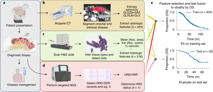
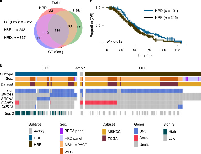
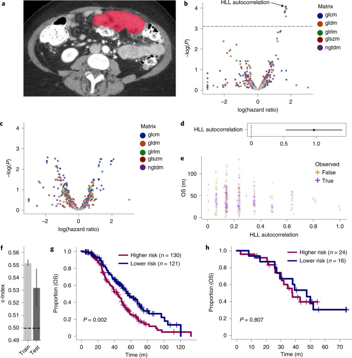
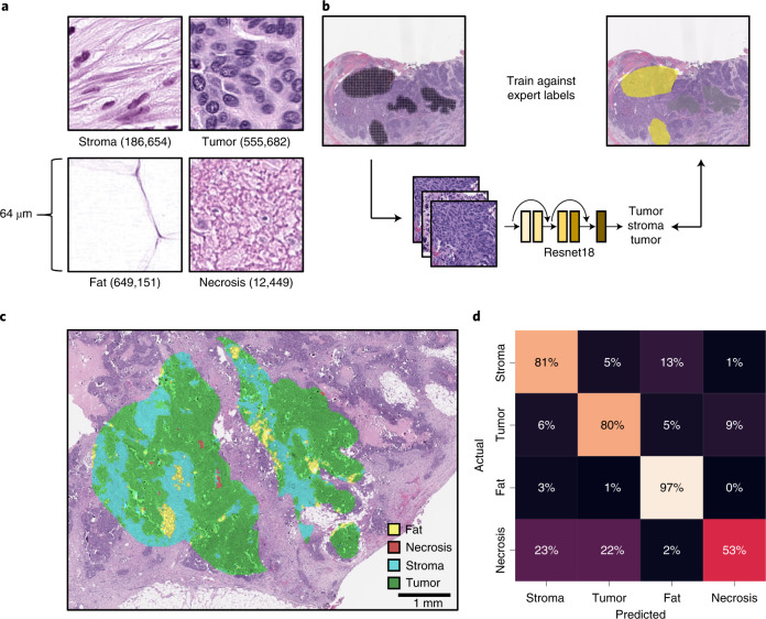
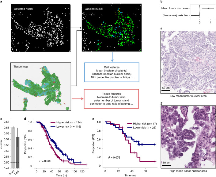
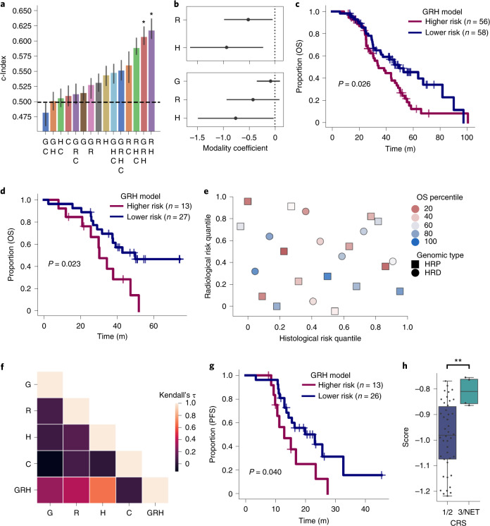
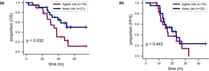
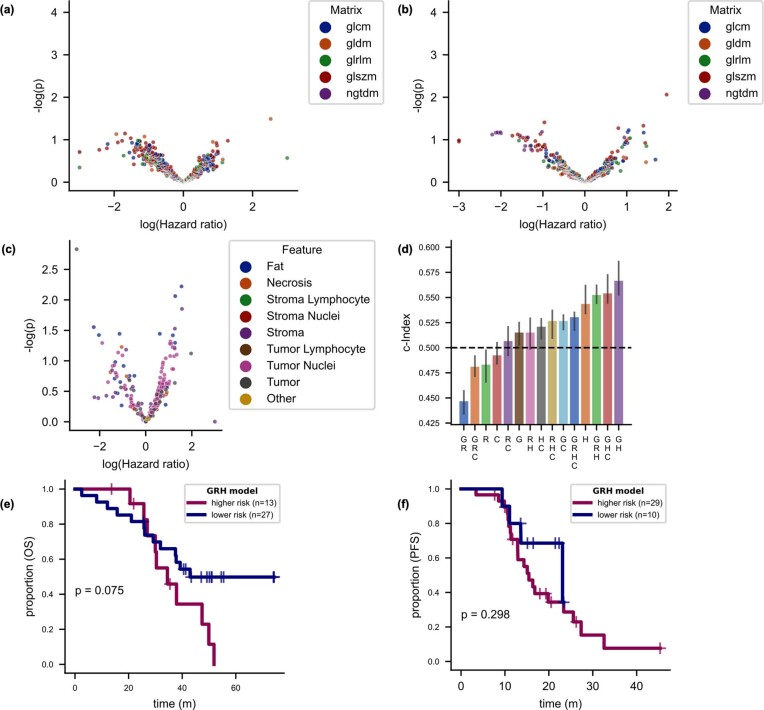
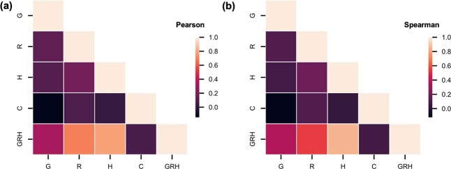
Patients with high-grade serous ovarian cancer suffer poor prognosis and variable response to treatment. Known prognostic factors for this disease include homologous recombination deficiency status, age, pathological stage and residual disease status after debulking surgery. Recent work has highlighted important prognostic information captured in computed tomography and histopathological specimens, which can be exploited through machine learning. However, little is known about the capacity of combining features from these disparate sources to improve prediction of treatment response. Here, we assembled a multimodal dataset of 444 patients with primarily late-stage high-grade serous ovarian cancer and discovered quantitative features, such as tumor nuclear size on staining with hematoxylin and eosin and omental texture on contrast-enhanced computed tomography, associated with prognosis. We found that these features contributed complementary prognostic information relative to one another and clinicogenomic features. By fusing histopathological, radiologic and clinicogenomic machine-learning models, we demonstrate a promising path toward improved risk stratification of patients with cancer through multimodal data integration.
Overview
The claims and statistics of this paper haven’t been checked yet.
Run the check — free, no account needed. It reads the open-access text and checks the sources it cites.
Integrity signals
Registry
Cites
Statistics
Figures
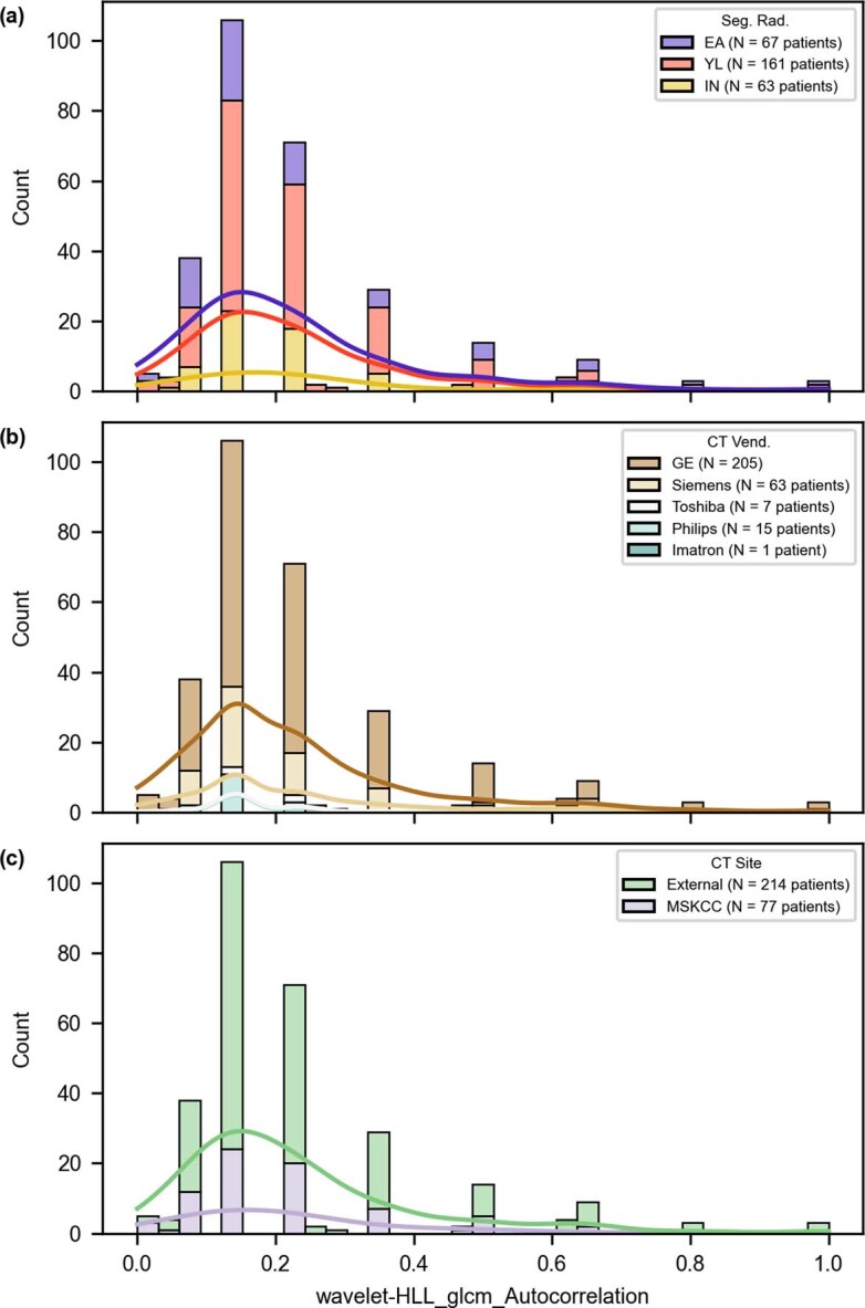
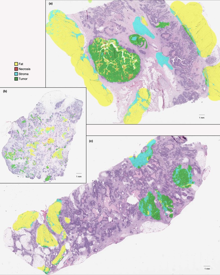
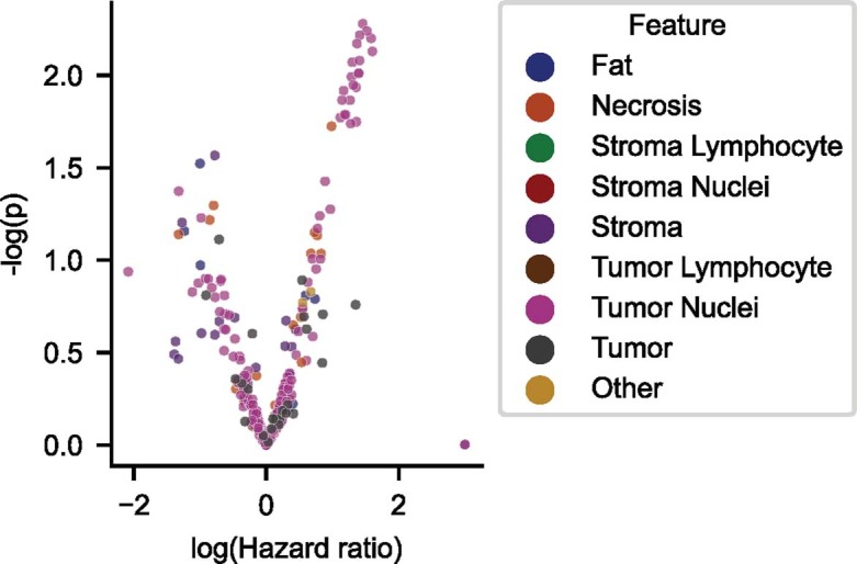
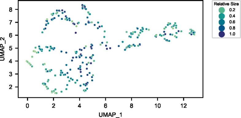
Verification
Claims the paper makes
The claims and statistics of this paper haven’t been checked yet.
Run the check — free, no account needed. It reads the open-access text and checks the sources it cites.
Claims other papers make about this one
Each is checked against this paper’s own text: does it say what the citing paper says it does?
The cited source says what the claim attributes to it.
In the citing paper
“Boehm et al. comprehensively characterized the multimodal datasets of high-grade serous ovarian cancer and proposed that a combination of histopathological, radiologic, and genomic features can better predict the prognosis of patients and aid in risk stratification [103].”
From Challenges in AI-driven Biomedical Multimodal Data Fusion and Analysis (2025) · cites this paper as [103]
In the citing paper
“Boehm and colleagues (170) used TCGA and an internal cohort to fuse genomic data, histopathology imaging, and radiology imaging to predict survival in high-grade serous ovarian cancer.”
From Artificial Intelligence in Oncology: Current Landscape, Challenges, and Future Directions (2024) · cites this paper as [170]
Self-check
Percentages, sums and reported differences re-computed from the paper’s own numbers.
The self-check needs the paper’s full text.
Citations
Cites
Controlling the False Discovery Rate: A Practical and Powerful Approach to Multiple Testing
Benjamini, Y., & Hochberg, Y. (1995) · Journal of the Royal Statistical Society Series B: Statistical Methodology · doi:10.1111/j.2517-6161.1995.tb02031.x · Cited by 109,482
Textural Features for Image Classification
Haralick, R. M., Shanmugam, K., & Dinstein, I. (1973) · IEEE Transactions on Systems, Man, and Cybernetics · doi:10.1109/tsmc.1973.4309314 · Cited by 22,886
Rudin, C. (2019) · Nature Machine Intelligence · doi:10.1038/s42256-019-0048-x · Cited by 10,561
QuPath: Open source software for digital pathology image analysis
Bankhead, P., Loughrey, M. B., Fernández, J. A., Dombrowski, Y., McArt, D. G., Dunne, P. D., McQuaid, S., Gray, R. T., Murray, L. J., Coleman, H. G., et al. (2017) · Scientific Reports · doi:10.1038/s41598-017-17204-5 · Cited by 8,908
Integrated genomic analyses of ovarian carcinoma
Perou, C. M. (2019) · Carolina Digital Repository (University of North Carolina at Chapel Hill) · doi:10.17615/hvp3-wg08 · Cited by 7,927
scikit-image: image processing in Python
(2014) · doi:10.7717/peerj.453 · Cited by 6,794
Computational Radiomics System to Decode the Radiographic Phenotype
(2017) · doi:10.1158/0008-5472.can-17-0339 · Cited by 6,593
Zwanenburg, A., Vallières, M., Abdalah, M. A., Aerts, H. J. W. L., Andrearczyk, V., Apte, A., Ashrafinia, S., Bakas, S., Beukinga, R. J., Boellaard, R., et al. (2020) · Radiology · doi:10.1148/radiol.2020191145 · Cited by 4,177
Liu, J., Lichtenberg, T., Hoadley, K. A., Poisson, L. M., Lazar, A. J., Cherniack, A. D., Kovatich, A. J., Benz, C. C., Levine, D. A., Lee, A. V., et al. (2018) · Cell · doi:10.1016/j.cell.2018.02.052 · Cited by 3,725
Self-citationThe repertoire of mutational signatures in human cancer
Alexandrov, L. B., Kim, J., Haradhvala, N. J., Huang, M. N., Tian Ng, A. W., Wu, Y., Boot, A., Covington, K. R., Gordenin, D. A., Bergstrom, E. N., et al. (2020) · Nature · doi:10.1038/s41586-020-1943-3 · Cited by 3,496
Zehir, A., Benayed, R., Shah, R. H., Syed, A., Middha, S., Kim, H. R., Srinivasan, P., Gao, J., Chakravarty, D., Devlin, S. M., et al. (2017) · Nature Medicine · doi:10.1038/nm.4333 · Cited by 3,380
Self-citationMaintenance Olaparib in Patients with Newly Diagnosed Advanced Ovarian Cancer
Moore, K., Colombo, N., Scambia, G., Kim, B.-G., Oaknin, A., Friedlander, M., Lisyanskaya, A., Floquet, A., Leary, A., Sonke, G. S., et al. (2018) · New England Journal of Medicine · doi:10.1056/nejmoa1810858 · Cited by 2,870
OncoKB: A Precision Oncology Knowledge Base
Chakravarty, D., Gao, J., Phillips, S. M., Kundra, R., Zhang, H., Wang, J., Rudolph, J. E., Yaeger, R. D., Soumerai, T. E., Nissan, M. H., et al. (2017) · JCO Precision Oncology · doi:10.1200/po.17.00011 · Cited by 2,783
Self-citationTexture analysis using gray level run lengths
Galloway, M. M. (1975) · Computer Graphics and Image Processing · doi:10.1016/s0146-664x(75)80008-6 · Cited by 2,168
Memorial Sloan Kettering-Integrated Mutation Profiling of Actionable Cancer Targets (MSK-IMPACT)
Cheng, D. T., Mitchell, T. N., Zehir, A., Shah, R. H., Benayed, R., Syed, A., Chandramohan, R., Liu, Z. Y., Won, H. H., Scott, S. N., et al. (2015) · The Journal of Molecular Diagnostics · doi:10.1016/j.jmoldx.2014.12.006 · Cited by 2,119
Cell Detection with Star-Convex Polygons
Schmidt, U., Weigert, M., Broaddus, C., & Myers, G. (2018) · Lecture Notes in Computer Science · doi:10.1007/978-3-030-00934-2_30 · Cited by 1,826
Fast wavelet transforms and numerical algorithms I
Beylkin, G., Coifman, R. R., & Rokhlin, V. (1991) · Communications on Pure and Applied Mathematics · doi:10.1002/cpa.3160440202 · Cited by 1,754
Rethinking ovarian cancer II: reducing mortality from high-grade serous ovarian cancer
Bowtell, D. D. L., Böhm, S., Ahmed, A. A., Aspuria, P.-J. P., Bast, R. C., Beral, V., Berek, J. S., Birrer, M. J., Blagden, S. P., Bookman, M. A., et al. (2015) · Nature reviews. Cancer · doi:10.1038/nrc4019 · Cited by 1,395
Texture analysis of SAR sea ice imagery using gray level co-occurrence matrices
Soh, L.-K., & Tsatsoulis, C. (1999) · IEEE Transactions on Geoscience and Remote Sensing · doi:10.1109/36.752194 · Cited by 1,238
Textural features corresponding to textural properties
Amadasun, M., & King, R. A. (1989) · IEEE Transactions on Systems Man and Cybernetics · doi:10.1109/21.44046 · Cited by 1,163
lifelines: survival analysis in Python
Davidson-Pilon, C. (2019) · The Journal of Open Source Software · doi:10.21105/joss.01317 · Cited by 1,071
Chang, M. T., Asthana, S., Gao, S. P., Lee, B. H., Chapman, J. S., Kandoth, C., Gao, J., Socci, N. D., Solit, D. B., Olshen, A. B., et al. (2016) · Nature Biotechnology · doi:10.1038/nbt.3391 · Cited by 808
Self-citationQuPath: Open source software for digital pathology image analysisPreprint
Bankhead, P., Loughrey, M. B., Fernández, J. A., et al. (2017) · bioRxiv (Cold Spring Harbor Laboratory) · doi:10.1101/099796 · Cited by 808
Popova, T. G., Manié, É., Rieunier, G., Caux‐Moncoutier, V., Tirapo, C., Dubois, T., Delattre, O., Sigal‐Zafrani, B., Bollet, M. A., Longy, M., et al. (2012) · Cancer Research · doi:10.1158/0008-5472.can-12-1470 · Cited by 683
Harnessing multimodal data integration to advance precision oncology
Boehm, K. M., Khosravi, P., Vanguri, R., Gao, J., & Shah, S. P. (2022) · Nature Reviews Cancer · doi:10.1038/s41568-021-00408-3 · Cited by 662
Self-citationPan-cancer computational histopathology reveals mutations, tumor composition and prognosis
Fu, Y., Jung, A. W., Viñas, R., González, S., Vöhringer, H. S., Shmatko, A., Yates, L. R., Jimenez‐Liñan, M., Moore, L., & Gerstung, M. (2020) · Nature Cancer · doi:10.1038/s43018-020-0085-8 · Cited by 655
Multi-omic machine learning predictor of breast cancer therapy response
Sammut, S.-J., Crispin-Ortuzar, M., Chin, S.-F., Provenzano, E., Bardwell, H. A., Ma, W., Cope, W., Dariush, A., Dawson, S.-J., Abraham, J. E., et al. (2022) · Nature · doi:10.1038/s41586-021-04278-5 · Cited by 654
What Makes Training Multi-modal Classification Networks Hard?
Wang, W., Tran, D., & Feiszli, M. (2020) · 2020 IEEE/CVF Conference on Computer Vision and Pattern Recognition (CVPR) · doi:10.1109/cvpr42600.2020.01271 · Cited by 588
Deep learning-based classification of mesothelioma improves prediction of patient outcome
Courtiol, P., Maussion, C., Moarii, M., Pronier, E., Pilcer, S., Sefta, M., Manceron, P., Toldo, S., Zaslavskiy, M., Le Stang, N., et al. (2019) · Nature Medicine · doi:10.1038/s41591-019-0583-3 · Cited by 544
The Repertoire of Mutational Signatures in Human CancerPreprint
Alexandrov, L. B., Kim, J., Haradhvala, N. J., Huang, M. N., Ng, A. W. T., Wu, Y., Boot, A., Covington, K. R., Gordenin, D. A., Bergstrom, E. N., et al. (2018) · bioRxiv (Cold Spring Harbor Laboratory) · doi:10.1101/322859 · Cited by 529
Prevalence of Homologous Recombination–Related Gene Mutations Across Multiple Cancer Types
Heeke, A. L., Pishvaian, M. J., Lynce, F. C., Xiu, J., Brody, J. R., Chen, W.-J., Baker, T. M., Marshall, J. L., & Isaacs, C. J. (2018) · JCO Precision Oncology · doi:10.1200/po.17.00286 · Cited by 477
Copy number signatures and mutational processes in ovarian carcinoma
Macintyre, G., Goranova, T., Silva, D. D., Ennis, D. P., Piskorz, A., Eldridge, M., Sie, D., Lewsley, L.-A., Hanif, A., Wilson, C. A., et al. (2018) · Nature Genetics · doi:10.1038/s41588-018-0179-8 · Cited by 434
Neighboring gray level dependence matrix for texture classification
Sun, C., & Wee, W. G. (1983) · Computer Vision Graphics and Image Processing · doi:10.1016/0734-189x(83)90032-4 · Cited by 415
Accelerating Discovery of Functional Mutant Alleles in Cancer
Chang, M. T., Shrestha-Bhattarai, T., Schram, A. M., Bielski, C. M., Donoghue, M. T. A., Jonsson, P., Chakravarty, D., Phillips, S. M., Kandoth, C., Penson, A. V., et al. (2017) · Cancer Discovery · doi:10.1158/2159-8290.cd-17-0321 · Cited by 413
Self-citationInterfaces of Malignant and Immunologic Clonal Dynamics in Ovarian Cancer
Zhang, A. W., McPherson, A., Milne, K., Kroeger, D. R., Hamilton, P. T., Miranda, A., Funnell, T., Gierc, N. S., de Souza, C. P. E., Laan, S., et al. (2018) · Cell · doi:10.1016/j.cell.2018.03.073 · Cited by 353
Self-citationOvarian cancer mutational processes drive site-specific immune evasion
Vázquez-Garćıa, I., Uhlitz, F., Ceglia, N., Lim, J. L., Wu, M. K. Y., Mohibullah, N., Niyazov, J., Ruiz, A. E. B., Boehm, K. M., Bojilova, V., et al. (2022) · Nature · doi:10.1038/s41586-022-05496-1 · Cited by 329
Self-citationDetecting the mutational signature of homologous recombination deficiency in clinical samples
Gulhan, D., Lee, J. J.-K., Melloni, G. E. M., Cortés‐Ciriano, I., & Park, P. J. (2019) · Nature Genetics · doi:10.1038/s41588-019-0390-2 · Cited by 318
Diao, J. A., Wang, J. K., Chui, W. F., Mountain, V., Gullapally, S. C., Srinivasan, R., Mitchell, R. N., Glass, B., Hoffman, S., Rao, S. K., et al. (2021) · Nature Communications · doi:10.1038/s41467-021-21896-9 · Cited by 289
Pan-cancer analysis of bi-allelic alterations in homologous recombination DNA repair genes
Riaz, N., Blecua, P., Lim, R. S., Shen, R., Higginson, D. S., Weinhold, N., Norton, L., Weigelt, B., Powell, S. N., & Reis-Filho, J. S. (2017) · Nature Communications · doi:10.1038/s41467-017-00921-w · Cited by 249
Self-citationWhole slide imaging equivalency and efficiency study: experience at a large academic center
Hanna, M. G., Reuter, V. E., Hameed, M., Tan, L. K., Chiang, S., Sigel, C., Hollmann, T. J., Giri, D. D., Samboy, J., Moradel, C., et al. (2019) · Modern Pathology · doi:10.1038/s41379-019-0205-0 · Cited by 215
Lu, H., Arshad, M., Thornton, A., Avesani, G., Cunnea, P., Curry, E. W., Kanavati, F., Liang, J., Nixon, K., Williams, S. T., et al. (2019) · Nature Communications · doi:10.1038/s41467-019-08718-9 · Cited by 213
SHAPE AND TEXTURE INDEXES APPLICATION TO CELL NUCLEI CLASSIFICATION
THIBAULT, G., Fertil, B., Navarro, C. L., Pereira, S., Cau, P., Lévy, N., Séqueira, J., & MARI, J.-L. (2013) · International Journal of Pattern Recognition and Artificial Intelligence · doi:10.1142/s0218001413570024 · Cited by 198
Wang, S., Liu, Z., Rong, Y., Zhou, B., Bai, Y., Wei, W., Wei, W., Wang, M., Guo, Y., & Tian, J. (2018) · Radiotherapy and Oncology · doi:10.1016/j.radonc.2018.10.019 · Cited by 175
Rizzo, S., Botta, F., Raimondi, S., Origgi, D., Buscarino, V., Colarieti, A., Tomao, F., Aletti, G. D., Zanagnolo, V. L., Grande, M. D., et al. (2018) · European Radiology · doi:10.1007/s00330-018-5389-z · Cited by 131
Integrated genomic analyses of ovarian carcinoma
The Cancer Genome Atlas Research Network (2011) · Nature · doi:10.1038/nature10166 · Cited by 129
Vargas, H. A., Veeraraghavan, H., Miccò, M., Nougaret, S., Lakhman, Y., Meier, A. A., Sosa, R. E., Soslow, R. A., Levine, D. A., Weigelt, B., et al. (2017) · European Radiology · doi:10.1007/s00330-017-4779-y · Cited by 121
Self-citationGallagher, D. J., Konner, J. A., Bell-McGuinn, K. M., Bhatia, J., Sabbatini, P. J., Aghajanian, C. A., Offit, K., Barakat, R. R., Spriggs, D. R., & Kauff, N. D. (2010) · Annals of Oncology · doi:10.1093/annonc/mdq577 · Cited by 118
TCIA: An information resource to enable open science
Prior, F., Clark, K., Commean, P. K., Freymann, J., Jaffe, C. C., Kirby, J., Moore, S., Smith, K., Tarbox, L., Vendt, B. A., et al. (2013) · Annual International Conference of the IEEE Engineering in Medicine and Biology Society (EMBC) · doi:10.1109/embc.2013.6609742 · Cited by 114
Gorodnova, T. V., Соколенко, А. П., Ivantsov, A. O., Iyevleva, A. G., Suspitsin, E. N., Алексахина, С. Н., Yanus, G. A., Togo, A. V., Maximov, S. Y., & Имянитов, Е. Н. (2015) · Cancer Letters · doi:10.1016/j.canlet.2015.08.028 · Cited by 103
Pan-cancer computational histopathology reveals mutations, tumor composition and prognosisPreprint
Fu, Y., Jung, A. W., Viñas, R., et al. (2019) · bioRxiv (Cold Spring Harbor Laboratory) · doi:10.1101/813543 · Cited by 95
Copy-number signatures and mutational processes in ovarian carcinomaPreprint
Macintyre, G., Goranova, T., Silva, D. D., et al. (2017) · bioRxiv (Cold Spring Harbor Laboratory) · doi:10.1101/174201 · Cited by 94
Meier, A., Veeraraghavan, H., Nougaret, S., Lakhman, Y., Sosa, R. E., Soslow, R. A., Sutton, E. J., Hricak, H., Sala, E., & Vargas, H. A. (2018) · Abdominal Radiology · doi:10.1007/s00261-018-1840-5 · Cited by 73
Self-citationFunnell, T., Zhang, A. W., Grewal, D. S., McKinney, S. E., Bashashati, A., Wang, Y. K., & Shah, S. P. (2019) · PLoS Computational Biology · doi:10.1371/journal.pcbi.1006799 · Cited by 63
Self-citationWei, W., Liu, Z., Rong, Y., Zhou, B., Bai, Y., Wei, W., Wang, S., Wang, M., Guo, Y., & Tian, J. (2019) · Frontiers in Oncology · doi:10.3389/fonc.2019.00255 · Cited by 60
Zargari, A., Du, Y., Heidari, M., Thai, T., Gunderson, C. C., Moore, K. N., Mannel, R. S., Liu, H., Zheng, B., & Qiu, Y. (2018) · Physics in Medicine and Biology · doi:10.1088/1361-6560/aad3ab · Cited by 45
Rizzo, S., Manganaro, L., Dolciami, M., Gasparri, M. L., Papadia, A., & Grande, F. D. (2021) · Cancers · doi:10.3390/cancers13030573 · Cited by 39
The Landscape of Somatic Genetic Alterations in Breast Cancers from CHEK2 Germline Mutation Carriers
Mandelker, D. L., Kumar, R., Pei, X., Selenica, P., Setton, J. S., Arunachalam, S., Ceyhan‐Birsoy, O., Brown, D. N., Norton, L., Robson, M. E., et al. (2019) · JNCI Cancer Spectrum · doi:10.1093/jncics/pkz027 · Cited by 36
Self-citationCurrent status and future directions of ovarian cancer prognostic models
Kobayashi, Y., Banno, K., & Aoki, D. (2021) · Journal of Gynecologic Oncology · doi:10.3802/jgo.2021.32.e34 · Cited by 14
Vázquez-Garćıa, I., Uhlitz, F., Ceglia, N., et al. (2021) · bioRxiv (Cold Spring Harbor Laboratory) · doi:10.1101/2021.08.24.454519 · Cited by 7
Cited by
Sorted by citations
Multistain deep learning for prediction of prognosis and therapy response in colorectal cancer
Foersch, S., Glasner, C., Woerl, A.-C., Eckstein, M., Wagner, D.-C., Schulz, S., Kellers, F., Fernandez, A., Tserea, K., Kloth, M., et al. (2023) · Nature Medicine · doi:10.1038/s41591-022-02134-1 · Cited by 251
A guide to artificial intelligence for cancer researchers
Pérez-López, R., Laleh, N. G., Mahmood, F., & Kather, J. N. (2024) · Nature reviews. Cancer · doi:10.1038/s41568-024-00694-7 · Cited by 227
Shaik, T., Tao, X., Li, L., Xie, H., & Velasquez, J. D. (2023) · Information Fusion · doi:10.1016/j.inffus.2023.102040 · Cited by 228
Artificial Intelligence in Oncology: Current Landscape, Challenges, and Future Directions
Lotter, W., Hassett, M. J., Schultz, N., Kehl, K. L., Van Allen, E. M., & Cerami, E. (2024) · Cancer Discovery · doi:10.1158/2159-8290.cd-23-1199 · Cited by 196
Metadata
- Authors
- Boehm, K. M., Aherne, E. A., Ellenson, L., Nikolovski, I., Alghamdi, M., Vázquez-García, I., Zamarin, D., Long Roche, K., Liu, Y., Patel, D., Aukerman, A., Pasha, A., Rose, D., Selenica, P., Causa Andrieu, P. I., Fong, C., Capanu, M., Reis-Filho, J. S., Vanguri, R., Veeraraghavan, H., Gangai, N., Sosa, R., Leung, S., McPherson, A., Gao, J., MSK MIND Consortium, Lakhman, Y., & Shah, S. P.
- Affiliations
- Memorial Sloan Kettering Cancer Center (US)
- Corresponding author
- Lakhman, Yulia
- Shah, Sohrab P.
- ORCID
- Boehm, Kevin M.
- Aherne, Emily A.
- Ellenson, Lora
- Nikolovski, Ines
- Alghamdi, Mohammed
- Vázquez-García, Ignacio
- Zamarin, Dmitriy
- Long Roche, Kara
- Liu, Ying
- Patel, Druv
- Aukerman, Andrew
- Rose, Doori
- Selenica, Pier
- Fong, Chris
- Capanu, Marinela
- Reis-Filho, Jorge S.
- Vanguri, Rami
- Veeraraghavan, Harini
- Gangai, Natalie
- McPherson, Andrew
- Gao, JianJiong
- Lakhman, Yulia
- Shah, Sohrab P.
- Venue
- Nature Cancer
- Published
- 2022-06-28
- Volume
- 3
- Issue
- 6
- Pages
- 723-733
- ISSN
- 2662-1347 (ISSN-L)
- PMC
- PMC9239907
- OpenAlex
- W4283645969
- Cited by
- 357
- References
- 54
- Citations by year
- 2026: 76 · 2025: 118 · 2024: 94 · 2023: 59 · 2022: 9
- FWCI
- 59.41
- Type
- journal article
- Language
- en
- Open access
- hybrid
- doi.org
- Locations
- Nature Cancer (publishedVersion, cc-by)
- PubMed Central (publishedVersion, cc-by)
- PubMed (publishedVersion)
- Funders
- U.S. Department of Health & Human Services | NIH | National Institute of General Medical Sciences (T32GM007739)
- U.S. Department of Health & Human Services | NIH | NCI | Division of Cancer Epidemiology and Genetics, National Cancer Institute (P30CA008748)
- Grayer Fellowship (MSKCC) Cycle for Survival
- Susan G. Komen Scholars Program Cycle for Survival
- Topics
- Health Sciences › Medicine › Oncology › Ovarian cancer diagnosis and treatment
- Health Sciences › Medicine › Radiology, Nuclear Medicine and Imaging › Radiomics and Machine Learning in Medical Imaging
- Physical Sciences › Computer Science › Artificial Intelligence › AI in cancer detection
- Keywords
- high-grade serous ovarian cancer, multimodal data integration, risk stratification, prognostic factors, treatment response prediction, homologous recombination deficiency, H&E staining, contrast-enhanced CT, histopathology
- MeSH terms
- Machine Learning, Female, Humans, Ovarian Neoplasms, Cystadenocarcinoma, Serous, Risk Assessment
About these checks
Registry, retraction, Cites and statistics results are computed, not judged, with one exception: a printed reference that no index lists is read once by a model before it counts as a citation error. Claims are extracted by a model and kept only when their quote appears verbatim in the text; each cited source is then checked, with a model’s help, for whether it says what the claim relies on. Those verdicts can be wrong — read the claim’s quote and the cited source before relying on one.
Statistics and arithmetic are recomputed, not judged.
Confidence bands are shown only for fields calibrated on our annotated test set. None is calibrated yet, so no band is shown.
What counts as a claim ›How we measure confidence ›How we check this ›
Are you an author, or do you see a problem with this page? Request a review
